Analysis of an Iterative Approach to Determine the Current on the Straight Infinite Wire Above Ground

An iterative approach which was recently applied to approximate the reflection and scattering coefficients of transmission line ports is analyzed. The iterative solution for the current on an infinite wire above ground is compared to the exact solution. The example is chosen since it is one of the few problems where an exact solution exists. The wire is excited by a lumped voltage source or a plane wave. The convergence of the iterative approach is shown. It can be concluded that the zeroth iteration, which is the classical transmission line solution, coincides with the general transverse electromagnetic mode. Furthermore, it is shown that the first iteration is a very good approximation of the radiation and leaky modes, that occur in the close neighborhood around the lumped source.

1 Introduction

Transmission lines play an important part in many branches of electrical engineering. Hence, it is of great interest to understand the propagation of waves along transmission lines and develop analytic methods to determine the currents on wires.

Recently, an iterative approach was developed for thin wires above ground and applied to many examples (see e.g. Rachidi and Tkachenko, 2008; Middelstaedt et al., 2015, 2018). The iterative approach can be seen as an extension to the classical transmission line approximation, which is restricted to uniform transmission lines and to wavelengths much larger than the transverse dimensions of the transmission lines. After only one iteration the iterative approach already yields accurate results for infinite and semi-infinite problems respecting the non-uniformity of the wire.

Due to the success of the iterative approach, questions that arise are:

1. Does the iterative approach converge if more iterations are used?

2. What is the interpretation of the solution of each iteration step?

A first step in answering these fundamental questions is done in this paper. The questions are answered using the example of the infinite wire above ground excited by a lumped voltage source and a plane wave. This specific problem is chosen since its exact analytic solution is available for comparison.

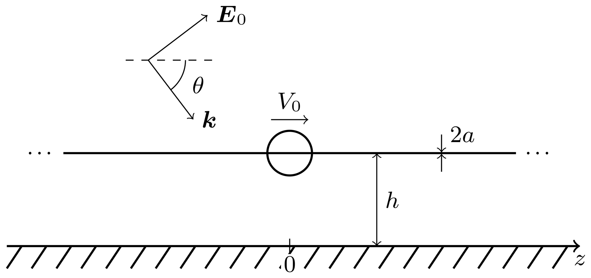
Figure 1 shows the thin wire above an infinite, planar, perfectly electrically conducting ground. It is assumed that the radius a of the wire is much smaller than its height h above ground. Hence, the thin wire approximation can be applied. The wire is either excited by a lumped voltage source with amplitude V₀ or by a plane wave with wave number $k=\Vert \mathit{k}\Vert$ and electric field vector E₀. The angle of incident is denoted by θ and is defined as shown in Fig. 1.

The current density vector, that arises due to the sources, is defined to be pointing in the positive z-direction. The corresponding current is denoted by I. The current I and the electric scalar potential Φ can both be determined using the so call mixed potential integral equations (MPIE). The MPIE are derived in many publications e.g. in Nitsch and Tkachenko (2010),

$$\begin{array}{}\text{(1a)}& {\displaystyle \frac{\partial }{\partial z}}\mathrm{\Phi }\left(z\right)+\mathrm{j}\mathit{\omega }{\displaystyle \frac{{\mathit{\mu }}_{\mathrm{0}}}{\mathrm{4}\mathit{\pi }}}\mathcal{G}I\left(z\right)& {\displaystyle }=E_{\tan }\left(z\right)\text{(1b)}& {\displaystyle }\mathcal{G}{\displaystyle \frac{\partial }{\partial z}}I\left(z\right)+\mathrm{4}\mathit{\pi }\mathrm{j}\mathit{\omega }{\mathit{\epsilon }}_{\mathrm{0}}\mathrm{\Phi }\left(z\right)& {\displaystyle }=\mathrm{0}.\end{array}$$

The operator 𝒢 is defined as a convolution integral

$$\begin{array}{}\text{(2)}& \mathcal{G}I\left(z\right)=\underset{-\mathrm{\infty }}{\overset{\mathrm{\infty }}{\int }}\mathrm{d}{z}^{\prime }G(z-z^{\prime })I\left(z^{\prime }\right)\end{array}$$

with the Green's function for the half space

$$\begin{array}{}\text{(3)}& G\left(z\right)={\displaystyle \frac{\exp (-\mathrm{j}k\sqrt{z^{\mathrm{2}}+a^{\mathrm{2}}})}{\sqrt{z^{\mathrm{2}}+a^{\mathrm{2}}}}}-{\displaystyle \frac{\exp (-\mathrm{j}k\sqrt{z^{\mathrm{2}}+\mathrm{4}{h}^{\mathrm{2}}})}{\sqrt{z^{\mathrm{2}}+\mathrm{4}{h}^{\mathrm{2}}}}}.\end{array}$$

The following relation holds for the angular frequency ω, the permittivity ε₀, and the permeability μ₀

$$\begin{array}{}\text{(4)}& k=\mathit{\omega }\sqrt{{\mathit{\mu }}_{\mathrm{0}}{\mathit{\epsilon }}_{\mathrm{0}}}.\end{array}$$

The tangential electric field on the surface of the wire E_tan(z) depends on the kind of excitation. For the two considered cases it is given as

$$\begin{array}{}\text{(5)}& E_{\tan }=\left\{\begin{array}{ll}{V}_{\mathrm{0}}\mathit{\delta }\left(z\right)& \text{lumped voltage source}\\ E_z\exp (-\mathrm{j}{k}_{\mathit{\theta }}z)& \text{plane wave}\end{array}\right.\end{array}$$

with

$$\begin{array}{}\text{(6)}& {\displaystyle }{E}_z& {\displaystyle }=\mathrm{2}\mathrm{j}\Vert {\mathit{E}}_{\mathrm{0}}\Vert \sin \left(\mathit{\theta }\right)\sin \left(kh\sin \right(\mathit{\theta }\left)\right)\text{(7)}& {\displaystyle }{k}_{\mathit{\theta }}& {\displaystyle }=k\cos \left(\mathit{\theta }\right).\end{array}$$

The delta distribution is denoted by δ.

Figure 1 Infinite wire above ground with lumped voltage source and plane wave excitation.

Usually, the goal is to solve equations similar to Eq. (1) for the current I as in Leviatan and Adams (1982), Rachidi and Tkachenko (2008), and Middelstaedt et al. (2015, 2018). It is possible to find the exact solution for the straight infinite wire above ground. For more practical cases there are no exact analytic solutions but only approximations. The iterative approach yields one of these approximations.

In the following the exact solution and the iterative one are derived for the described example. The convergence of the iterative approach is analyzed. Furthermore, the iterative solution is interpreted by comparing it to the exact one.

2 Exact Solution

The problem of the infinite wire above ground is similar to the two wire transmission line in free space, which is dealt with in Schelkunoff (1956), Marin (1975), and Leviatan and Adams (1982). In Marin (1975) the focus lies on the determination of the electromagnetic fields that propagate along the wires in time domain. In Leviatan and Adams (1982) the authors focus only on the transverse electromagnetic (TEM) and leaky modes and ignore the radiation mode. Therefore, the solution for the current along the wire is derived here again with the focus on the current and all modes.

To solve Eq. (1) it is convenient to apply the Fourier transform. The Fourier transform and its inverse, which is marked with a tilde, are defined as

$$\begin{array}{}\text{(8)}& {\displaystyle }\stackrel{\mathrm{̃}}{I}\left(k_z\right)& {\displaystyle }=\underset{-\mathrm{\infty }}{\overset{\mathrm{\infty }}{\int }}\mathrm{d}zI\left(z\right)\exp (-\mathrm{j}{k}_{z}z)\text{(9)}& {\displaystyle }I\left(z\right)& {\displaystyle }={\displaystyle \frac{\mathrm{1}}{\mathrm{2}\mathit{\pi }}}\underset{-\mathrm{\infty }}{\overset{\mathrm{\infty }}{\int }}\mathrm{d}{k}_z\stackrel{\mathrm{̃}}{I}\left(k_z\right)\exp \left(\mathrm{j}{k}_{z}z\right).\end{array}$$

Fortunately, the transform of the Green's function G is known (see Nitsch and Tkachenko, 2002a)

$$\begin{array}{}\text{(10)}& \stackrel{\mathrm{̃}}{G}\left(k_z\right)=\left\{\begin{array}{ll}\begin{array}{rl}{\displaystyle }\mathrm{2}[& {\displaystyle }{K}_{\mathrm{0}}\left(a\sqrt{k_z^{\mathrm{2}}-k^{\mathrm{2}}}\right)\\ {\displaystyle }& {\displaystyle }-K_{\mathrm{0}}\left(\mathrm{2}h\sqrt{k_z^{\mathrm{2}}-k^{\mathrm{2}}}\right)]\end{array}& \text{for }{k}_z^{\mathrm{2}}\ne k^{\mathrm{2}}\\ \mathrm{2}\ln \left(\frac{\mathrm{2}h}{a}\right)& \text{for }{k}_z^{\mathrm{2}}=k^{\mathrm{2}}\end{array}\right.\end{array}$$

where K_m denotes the modified Bessel function of the second kind and order m.

After some mathematical manipulations the current I and its transform are found to be

$$\begin{array}{}\text{(11)}& {\displaystyle }\stackrel{\mathrm{̃}}{I}\left(k_z\right)& {\displaystyle }=\mathrm{4}\mathit{\pi }\mathrm{j}\mathit{\omega }{\mathit{\epsilon }}_{\mathrm{0}}{\displaystyle \frac{{\stackrel{\mathrm{̃}}{E}}_{\tan }\left(k_z\right)}{(k_z^{\mathrm{2}}-k^{\mathrm{2}})\stackrel{\mathrm{̃}}{G}\left(k_z\right)}}\text{(12)}& {\displaystyle }I\left(z\right)& {\displaystyle }=\mathrm{2}\mathrm{j}k\sqrt{{\displaystyle \frac{{\mathit{\epsilon }}_{\mathrm{0}}}{{\mathit{\mu }}_{\mathrm{0}}}}}\underset{-\mathrm{\infty }}{\overset{\mathrm{\infty }}{\int }}\mathrm{d}{k}_z{\displaystyle \frac{{\stackrel{\mathrm{̃}}{E}}_{\tan }\left(k_z\right)\exp \left(\mathrm{j}{k}_{z}z\right)}{(k_z^{\mathrm{2}}-k^{\mathrm{2}})\stackrel{\mathrm{̃}}{G}\left(k_z\right)}}.\end{array}$$

With Eq. (12) an explicit expression is given for the current that arises due to the excitation E_tan(z). Depending on the Fourier transform of the excitation ${\stackrel{\mathrm{̃}}{E}}_{\tan }\left(k_z\right)$ the integral can be solved. The transforms of the excitations given in Eq. (5) are

$$\begin{array}{}\text{(13)}& {\stackrel{\mathrm{̃}}{E}}_{\tan }\left(k_z\right)=\left\{\begin{array}{ll}{V}_{\mathrm{0}}& \text{lumped volt. source}\\ \mathrm{2}\mathit{\pi }{E}_z\mathit{\delta }(k_z+k_{\mathit{\theta }})& \text{plane wave.}\end{array}\right.\end{array}$$

Hence, the solution resulting from the plane wave excitation is simply

$$\begin{array}{}\text{(14)}& {\displaystyle }{I}_{\mathrm{pw}}\left(z\right)& {\displaystyle }=\mathrm{4}\mathit{\pi }\mathrm{j}k{E}_z\sqrt{{\displaystyle \frac{{\mathit{\epsilon }}_{\mathrm{0}}}{{\mathit{\mu }}_{\mathrm{0}}}}}{\displaystyle \frac{\exp (-\mathrm{j}{k}_{\mathit{\theta }}z)}{(k_{\mathit{\theta }}^{\mathrm{2}}-k^{\mathrm{2}})\stackrel{\mathrm{̃}}{G}\left(k_{\mathit{\theta }}\right)}}\text{(15)}& {\displaystyle }& {\displaystyle }=\mathrm{8}\mathit{\pi }\sqrt{{\displaystyle \frac{{\mathit{\epsilon }}_{\mathrm{0}}}{{\mathit{\mu }}_{\mathrm{0}}}}}\Vert {\mathit{E}}_{\mathrm{0}}\Vert {\displaystyle \frac{\sin \left(kh\sin \right(\mathit{\theta }\left)\right)}{k\sin \left(\mathit{\theta }\right)}}{\displaystyle \frac{\exp (-\mathrm{j}{k}_{\mathit{\theta }}z)}{\stackrel{\mathrm{̃}}{G}\left(k_{\mathit{\theta }}\right)}}.\end{array}$$

2.1 Lumped Excitation

The procedure to obtain the solution for the lumped excitation is more advanced. The difficulty lies in the solution of the integral in Eq. (12), namely

$$\begin{array}{}\text{(16)}& I_{\mathrm{le}}\left(z\right)=\mathrm{2}\mathrm{j}k{V}_{\mathrm{0}}\sqrt{{\displaystyle \frac{{\mathit{\epsilon }}_{\mathrm{0}}}{{\mathit{\mu }}_{\mathrm{0}}}}}\underset{-\mathrm{\infty }}{\overset{\mathrm{\infty }}{\int }}\mathrm{d}{k}_z{\displaystyle \frac{\exp \left(\mathrm{j}{k}_{z}z\right)}{(k_z^{\mathrm{2}}-k^{\mathrm{2}})\stackrel{\mathrm{̃}}{G}\left(k_z\right)}}.\end{array}$$

The integral in Eq. (16) is analyzed using the residue theorem as in Marin (1975), Leviatan and Adams (1982). The variable k_z is assumed to be complex. Figure 2 shows the integration contour for Eq. (16) qualitatively in the complex plane for z>0. Since the problem is symmetric it is sufficient to only consider the solution for z>0, which will be done from now on.

The integrand has two branch cuts due to the square root in Eq. (10). The branch cuts in Fig. 2 connect the branch points at $k_z=\pm k$ via k_z=∞ (ref. Riemann sphere). The choice of the paths of the branch cuts originating from the fixed branch points is arbitrary. Here these specific branch cuts are chosen to allow a quick numerical integration along the branch cuts for later considerations.

Figure 2 Contour of integration for Eq. (16) for z>0 with poles in the complex plane k_z.

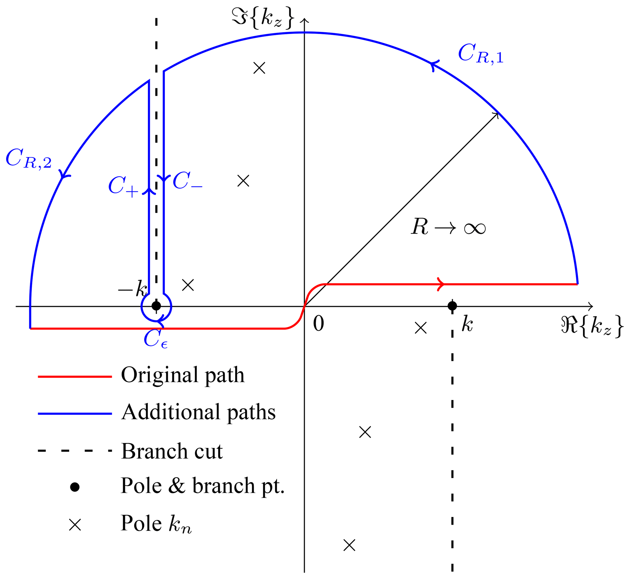
The residue theorem states that

$$\begin{array}{}\text{(17)}& {\displaystyle }\underset{-\mathrm{\infty }}{\overset{\mathrm{\infty }}{\int }}+\underset{C_{R,\mathrm{1}}}{\int }+\underset{C_{R,\mathrm{2}}}{\int }+\underset{C_{\mathit{ϵ}}}{\int }+\underset{C_{-}}{\int }+\underset{C_{+}}{\int }=\mathrm{2}\mathit{\pi }\mathrm{j}\sum _n\mathrm{Res}\left(k_n\right)\end{array}$$

where Res(k_n) denotes the residue of the integrand in Eq. (16) for the poles k_n inside the contour (see Fig. 2). The integration along the outer circle vanishes for R→∞ mainly due to the exponential function in the numerator and z>0.

$$\begin{array}{}\text{(18)}& \underset{R\to \mathrm{\infty }}{lim}(\underset{C_{R,\mathrm{1}}}{\int }+\underset{C_{R,\mathrm{2}}}{\int })=\mathrm{0}\end{array}$$

Hence,

$$\begin{array}{}\text{(19)}& \underset{-\mathrm{\infty }}{\overset{\mathrm{\infty }}{\int }}=-\underset{C_{\mathit{ϵ}}}{\int }+\mathrm{2}\mathit{\pi }\mathrm{j}\sum _n\mathrm{Res}\left(k_n\right)-(\underset{C_{-}}{\int }+\underset{C_{+}}{\int }).\end{array}$$

The integral around the branch point at $k_z=-k$ results in the TEM mode I_TEM(z). Each residue in Eq. (19) gives rise to leaky modes I_Leaky(z). The integration along the branch cut (in both directions) is connected to the radiation mode I_Rad(z). The total current can be expressed as a sum of these modes

$$\begin{array}{}\text{(20)}& I_{\mathrm{le}}\left(z\right)=I_{\mathrm{TEM}}\left(z\right)+I_{\mathrm{Leaky}}\left(z\right)+I_{\mathrm{Rad}}\left(z\right).\end{array}$$

The TEM and leaky modes are analyzed in great detail in Leviatan and Adams (1982). Their solution including the constant factor in front of the integral in Eq. (16) is

$$\begin{array}{}\text{(21)}& {\displaystyle }{I}_{\mathrm{TEM}}\left(z\right)& {\displaystyle }={\displaystyle \frac{V_{\mathrm{0}}}{\mathrm{2}{Z}_{\mathrm{C}}}}{\mathrm{e}}^{-\mathrm{j}kz}\text{(22)}& {\displaystyle }{I}_{\mathrm{Leaky}}\left(z\right)& {\displaystyle }=-\sum _n{\displaystyle \frac{V_{\mathrm{0}}}{\mathrm{2}{Z}_n}}{\mathrm{e}}^{\mathrm{j}{k}_{n}z}\end{array}$$

for z>0 with

$$\begin{array}{ll}\text{(23)}& {\displaystyle }{Z}_{\mathrm{C}}& {\displaystyle }={\displaystyle \frac{\ln \left(\frac{\mathrm{2}h}{a}\right)}{\mathrm{2}\mathit{\pi }}}\sqrt{{\displaystyle \frac{{\mathit{\mu }}_{\mathrm{0}}}{{\mathit{\epsilon }}_{\mathrm{0}}}}}{\displaystyle }{Z}_n& {\displaystyle }={\displaystyle \frac{k_n}{\mathrm{4}\mathit{\pi }k}}\sqrt{k_n^{\mathrm{2}}-k^{\mathrm{2}}}\sqrt{{\displaystyle \frac{{\mathit{\mu }}_{\mathrm{0}}}{{\mathit{\epsilon }}_{\mathrm{0}}}}}\left[a{K}_{\mathrm{1}}\right(-a\sqrt{k_n^{\mathrm{2}}-k^{\mathrm{2}}})\\ \text{(24)}& {\displaystyle }& {\displaystyle }-\mathrm{2}h{K}_{\mathrm{1}}(-\mathrm{2}h\sqrt{k_n^{\mathrm{2}}-k^{\mathrm{2}}})].\end{array}$$

The poles k_n (the roots of Eq. 10) that contribute to the solution are all located between the branch cut and the imaginary axis for this particularly chosen branch cut. There are poles, whose real part is smaller than −k. But they are part of a different Riemann surface. Hence, they are not part of the total current.

The radiation modes arise due to the integration along the branch cuts, specifically along the paths C₋ and C₊.

$$\begin{array}{}\text{(25)}& \begin{array}{rl}{I}_{\mathrm{Rad}}\left(z\right)& =-\mathrm{2}\mathrm{j}k{V}_{\mathrm{0}}\sqrt{{\displaystyle \frac{{\mathit{\epsilon }}_{\mathrm{0}}}{{\mathit{\mu }}_{\mathrm{0}}}}}(\underset{C_{-}}{\int }\mathrm{d}{k}_z{\displaystyle \frac{\exp \left(\mathrm{j}{k}_{z}z\right)}{(k_z^{\mathrm{2}}-k^{\mathrm{2}})\stackrel{\mathrm{̃}}{G}\left(k_z\right)}}\\ & +\underset{C_{+}}{\int }\mathrm{d}{k}_z{\displaystyle \frac{\exp \left(\mathrm{j}{k}_z\right)}{(k_z^{\mathrm{2}}-k^{\mathrm{2}})\stackrel{\mathrm{̃}}{G}\left(k_z\right)}})\end{array}\end{array}$$

With the definition of the branch cut (see Fig. 2) follows

$$\begin{array}{}\text{(26)}& {\displaystyle }\begin{array}{rl}{I}_{\mathrm{Rad}}\left(z\right)& =\mathrm{j}k{V}_{\mathrm{0}}\sqrt{{\displaystyle \frac{{\mathit{\epsilon }}_{\mathrm{0}}}{{\mathit{\mu }}_{\mathrm{0}}}}}\underset{-k}{\overset{-k+\mathrm{j}\mathrm{\infty }}{\int }}\mathrm{d}{k}_z{\displaystyle \frac{\exp \left(\mathrm{j}{k}_{z}z\right)}{(k_z^{\mathrm{2}}-k^{\mathrm{2}})}}[\\ & {\displaystyle \frac{\mathrm{1}}{K_{\mathrm{0}}(-a\sqrt{k_z^{\mathrm{2}}-k^{\mathrm{2}}})-K_{\mathrm{0}}(-\mathrm{2}h\sqrt{k_z^{\mathrm{2}}-k^{\mathrm{2}}})}}\\ & -{\displaystyle \frac{\mathrm{1}}{K_{\mathrm{0}}\left(a\sqrt{k_z^{\mathrm{2}}-k^{\mathrm{2}}}\right)-K_{\mathrm{0}}\left(\mathrm{2}h\sqrt{k_z^{\mathrm{2}}-k^{\mathrm{2}}}\right)}}]\end{array}\end{array}$$

The integral can be modified with the substitution $x=-\mathrm{j}(k_z+k)$, dk_z=j dx.

$$\begin{array}{}\text{(27)}& \begin{array}{rl}& I_{\mathrm{Rad}}\left(z\right)=-k{V}_{\mathrm{0}}\sqrt{{\displaystyle \frac{{\mathit{\epsilon }}_{\mathrm{0}}}{{\mathit{\mu }}_{\mathrm{0}}}}}{\mathrm{e}}^{-\mathrm{j}kz}\underset{\mathrm{0}}{\overset{\mathrm{\infty }}{\int }}\mathrm{d}x{\displaystyle \frac{\exp (-xz)}{-x(x+\mathrm{2}\mathrm{j}k)}}[\\ & {\displaystyle \frac{\mathrm{1}}{K_{\mathrm{0}}(-a\sqrt{-x(x+\mathrm{2}\mathrm{j}k)})-K_{\mathrm{0}}(-\mathrm{2}h\sqrt{-x(x+\mathrm{2}\mathrm{j}k)})}}\\ & -{\displaystyle \frac{\mathrm{1}}{K_{\mathrm{0}}\left(a\sqrt{-x(x+\mathrm{2}\mathrm{j}k)}\right)-K_{\mathrm{0}}\left(\mathrm{2}h\sqrt{-x(x+\mathrm{2}\mathrm{j}k)}\right)}}]\end{array}\end{array}$$

A solution for the latter integral is not known. But the integral is suitable for a fast numerical integration, especially for large z.

The treatment of the radiation mode is omitted in Leviatan and Adams (1982). In Marin (1975) the branch cut is chosen differently and hence, a different representation of the radiation mode is obtained.

The obtained exact solution is later used to interpret the iterative solution.

3 Iterative Approach

The iterative approach is described in many publications, e.g. Rachidi and Tkachenko (2008), Middelstaedt et al. (2016, 2018). The MPIE (Eq. 1) are modified to yield

$$\begin{array}{}\text{(28a)}& {\displaystyle \frac{\partial }{\partial z}}{\mathrm{\Phi }}^{\left(\mathrm{0}\right)}\left(z\right)+\mathrm{j}\mathit{\omega }{L}^{\prime }{I}^{\left(\mathrm{0}\right)}\left(z\right)& {\displaystyle }=E_{\tan }\left(z\right)\text{(28b)}& {\displaystyle \frac{\partial }{\partial z}}{I}^{\left(\mathrm{0}\right)}\left(z\right)+\mathrm{j}\mathit{\omega }{C}^{\prime }{\mathrm{\Phi }}^{\left(\mathrm{0}\right)}\left(z\right)& {\displaystyle }=\mathrm{0}\end{array}$$

for the iteration start and

$$\begin{array}{ll}{\displaystyle }& {\displaystyle \frac{\partial }{\partial z}}{\mathrm{\Phi }}^{\left(n\right)}\left(z\right)+\mathrm{j}\mathit{\omega }{L}^{\prime }{I}^{\left(n\right)}\left(z\right)=\mathrm{j}\mathit{\omega }{L}^{\prime }{I}^{(n-\mathrm{1})}\left(z\right)\\ \text{(29a)}& {\displaystyle }& {\displaystyle }-\mathrm{j}\mathit{\omega }{\displaystyle \frac{{\mathit{\mu }}_{\mathrm{0}}}{\mathrm{4}\mathit{\pi }}}\mathcal{G}{I}^{(n-\mathrm{1})}\left(z\right){\displaystyle }& {\displaystyle \frac{\partial }{\partial z}}{I}^{\left(n\right)}\left(z\right)+\mathrm{j}\mathit{\omega }{C}^{\prime }{\mathrm{\Phi }}^{\left(n\right)}\left(z\right)={\displaystyle \frac{\partial }{\partial z}}{I}^{(n-\mathrm{1})}\left(z\right)\\ \text{(29b)}& {\displaystyle }& {\displaystyle }-{\displaystyle \frac{\mathrm{1}}{\mathrm{2}\ln \left(\frac{\mathrm{2}h}{a}\right)}}\mathcal{G}{\displaystyle \frac{\partial }{\partial z}}{I}^{(n-\mathrm{1})}\left(z\right)\end{array}$$

for each iteration step with $n=\mathrm{1},\mathrm{2},\mathrm{\dots }$ and

$$\begin{array}{}\text{(30)}& {\displaystyle }{L}^{\prime }& {\displaystyle }={\displaystyle \frac{{\mathit{\mu }}_{\mathrm{0}}}{\mathrm{2}\mathit{\pi }}}\ln \left({\displaystyle \frac{\mathrm{2}h}{a}}\right)\text{(31)}& {\displaystyle }{C}^{\prime }& {\displaystyle }={\displaystyle \frac{\mathrm{2}\mathit{\pi }{\mathit{\epsilon }}_{\mathrm{0}}}{\ln \left(\frac{\mathrm{2}h}{a}\right)}}.\end{array}$$

The total current and total scalar potential are

$$\begin{array}{}\text{(32)}& {\displaystyle }I\left(z\right)& {\displaystyle }=I^{\left(\mathrm{0}\right)}\left(z\right)+I^{\left(\mathrm{1}\right)}\left(z\right)+\mathrm{\dots }\text{(33)}& {\displaystyle }\mathrm{\Phi }\left(z\right)& {\displaystyle }={\mathrm{\Phi }}^{\left(\mathrm{0}\right)}\left(z\right)+{\mathrm{\Phi }}^{\left(\mathrm{1}\right)}\left(z\right)+\mathrm{\dots }\end{array}$$

Equations (28) coincide with the classical telegrapher's equations. The equations for each iteration step (Eq. 29) have a similar form. But the source is the electric field emitted by the previously determined current I⁽ⁿ⁻¹⁾.

The equations can be solved using the Fourier transform as for the exact solution. The results are

$$\begin{array}{}\text{(34)}& {\displaystyle }{\stackrel{\mathrm{̃}}{I}}^{\left(\mathrm{0}\right)}\left(k_z\right)& {\displaystyle }=\mathrm{4}\mathit{\pi }\mathrm{j}\mathit{\omega }{\mathit{\epsilon }}_{\mathrm{0}}{\displaystyle \frac{{\stackrel{\mathrm{̃}}{E}}_{\tan }\left(k_z\right)}{(k_z^{\mathrm{2}}-k^{\mathrm{2}})\mathrm{2}\ln \left(\frac{\mathrm{2}h}{a}\right)}}\text{(35)}& {\displaystyle }{\stackrel{\mathrm{̃}}{I}}^{\left(n\right)}\left(k_z\right)& {\displaystyle }=(\mathrm{1}-{\displaystyle \frac{\stackrel{\mathrm{̃}}{G}\left(k_z\right)}{\mathrm{2}\ln \left(\frac{\mathrm{2}h}{a}\right)}}){\stackrel{\mathrm{̃}}{I}}^{(n-\mathrm{1})}\left(k_z\right)\text{(36)}& {\displaystyle }& {\displaystyle }=(\mathrm{1}-{\displaystyle \frac{\stackrel{\mathrm{̃}}{G}\left(k_z\right)}{\mathrm{2}\ln \left(\frac{\mathrm{2}h}{a}\right)}}{)}^n{\stackrel{\mathrm{̃}}{I}}^{\left(\mathrm{0}\right)}(k_z).\end{array}$$

Hence, the resulting total current is

$$\begin{array}{}\text{(37)}& {\displaystyle }\stackrel{\mathrm{̃}}{I}\left(k_z\right)& {\displaystyle }=\sum _{n=\mathrm{0}}^{\mathrm{\infty }}(\mathrm{1}-{\displaystyle \frac{\stackrel{\mathrm{̃}}{G}\left(k_z\right)}{\mathrm{2}\ln \left(\frac{\mathrm{2}h}{a}\right)}}{)}^n{\stackrel{\mathrm{̃}}{I}}^{\left(\mathrm{0}\right)}(k_z)\text{(38)}& {\displaystyle }& {\displaystyle }={\displaystyle \frac{\mathrm{4}\mathit{\pi }\mathrm{j}\mathit{\omega }{\mathit{\epsilon }}_{\mathrm{0}}{\stackrel{\mathrm{̃}}{E}}_{\tan }\left(k_z\right)}{(k_z^{\mathrm{2}}-k^{\mathrm{2}})\mathrm{2}\ln \left(\frac{\mathrm{2}h}{a}\right)}}\sum _{n=\mathrm{0}}^{\mathrm{\infty }}(\mathrm{1}-{\displaystyle \frac{\stackrel{\mathrm{̃}}{G}\left(k_z\right)}{\mathrm{2}\ln \left(\frac{\mathrm{2}h}{a}\right)}}{)}^n\end{array}$$

The geometric series converges if and only if

$$\begin{array}{}\text{(39)}& |\mathrm{1}-{\displaystyle \frac{\stackrel{\mathrm{̃}}{G}\left(k_z\right)}{\mathrm{2}\ln \left(\frac{\mathrm{2}h}{a}\right)}}|<\mathrm{1}.\end{array}$$

A parameter study found that Eq. (39) is always true as long as the thin wire approximation is applicable, meaning a≪h and $a\ll \mathrm{2}\mathit{\pi }/k$. Further details are illustrated in Appendix B. Hence, the total current from the iterative approach coincides with the exact result in Eq. (11) and therefore, converges to the correct solution.

For general wires it is not so straight forward to obtain the total current. Usually the zeroth and first iteration are determined analytically and the total current is approximated by the sum of those two currents. Therefore, this procedure is applied to this problem and the solutions are compared to the exact modes.

For the plane wave excitation it is straight forward to determine the currents $I_{\mathrm{pw}}^{\left(n\right)}\left(z\right)$ with Eqs. (34) and (36). They are

$$\begin{array}{}\text{(40)}& {\displaystyle }{I}_{\mathrm{pw}}^{\left(\mathrm{0}\right)}\left(z\right)& {\displaystyle }={\displaystyle \frac{\mathrm{8}\mathit{\pi }}{\mathrm{2}\ln \left(\frac{\mathrm{2}h}{a}\right)}}\sqrt{{\displaystyle \frac{{\mathit{\epsilon }}_{\mathrm{0}}}{{\mathit{\mu }}_{\mathrm{0}}}}}\Vert {\mathit{E}}_{\mathrm{0}}\Vert {\displaystyle \frac{\sin \left(kh\sin \right(\mathit{\theta }\left)\right)}{k\sin \left(\mathit{\theta }\right)}}{\mathrm{e}}^{-\mathrm{j}{k}_{\mathit{\theta }}z}\text{(41)}& {\displaystyle }{I}_{\mathrm{pw}}^{\left(n\right)}\left(z\right)& {\displaystyle }=(\mathrm{1}-{\displaystyle \frac{\stackrel{\mathrm{̃}}{G}\left(k_{\mathit{\theta }}\right)}{\mathrm{2}\ln \left(\frac{\mathrm{2}h}{a}\right)}}{)}^n{I}_{\mathrm{pw}}^{\left(\mathrm{0}\right)}(z).\end{array}$$

3.1 Lumped Excitation

To find the current of the zeroth and first iteration for the lumped excitation it is more convenient to not apply the Fourier transform. Thus, the complicated integral from the inverse Fourier transform is avoided.

It can be shown that

$$\begin{array}{}\text{(42)}& {\displaystyle \frac{\partial }{\partial z}}\mathcal{G}I\left(z\right)=\mathcal{G}{\displaystyle \frac{\partial }{\partial z}}I\left(z\right)\end{array}$$

by applying integration by parts. Decoupling Eqs. (28) and (29) then yields

$$\begin{array}{ll}\text{(43)}& {\displaystyle }& {\displaystyle }({\displaystyle \frac{{\partial }^{\mathrm{2}}}{\partial z^{\mathrm{2}}}}+k^{\mathrm{2}})I^{\left(\mathrm{0}\right)}\left(z\right)=-{\displaystyle \frac{\mathrm{4}\mathit{\pi }\mathrm{j}\mathit{\omega }{\mathit{\epsilon }}_{\mathrm{0}}}{\mathrm{2}\ln \left(\frac{\mathrm{2}h}{a}\right)}}{E}_{\tan }\left(z\right){\displaystyle }& {\displaystyle }({\displaystyle \frac{{\partial }^{\mathrm{2}}}{\partial z^{\mathrm{2}}}}+k^{\mathrm{2}})I^{\left(n\right)}\left(z\right)=({\displaystyle \frac{{\partial }^{\mathrm{2}}}{\partial z^{\mathrm{2}}}}+k^{\mathrm{2}})I^{(n-\mathrm{1})}\left(z\right)\\ \text{(44)}& {\displaystyle }& {\displaystyle }-{\displaystyle \frac{\mathrm{1}}{\mathrm{2}\ln \left(\frac{\mathrm{2}h}{a}\right)}}\mathcal{G}({\displaystyle \frac{{\partial }^{\mathrm{2}}}{\partial z^{\mathrm{2}}}}+k^{\mathrm{2}})I^{(n-\mathrm{1})}\left(z\right)\text{(45)}& {\displaystyle }& {\displaystyle }=(\mathrm{Id}-{\displaystyle \frac{\mathrm{1}}{\mathrm{2}\ln \left(\frac{\mathrm{2}h}{a}\right)}}\mathcal{G})({\displaystyle \frac{{\partial }^{\mathrm{2}}}{\partial z^{\mathrm{2}}}}+k^{\mathrm{2}})I^{(n-\mathrm{1})}\left(z\right)\text{(46)}& {\displaystyle }& {\displaystyle }=-{\displaystyle \frac{\mathrm{4}\mathit{\pi }\mathrm{j}\mathit{\omega }{\mathit{\epsilon }}_{\mathrm{0}}}{\mathrm{2}\ln \left(\frac{\mathrm{2}h}{a}\right)}}(\mathrm{Id}-{\displaystyle \frac{\mathrm{1}}{\mathrm{2}\ln \left(\frac{\mathrm{2}h}{a}\right)}}\mathcal{G}{)}^n{E}_{\tan }(z)\end{array}$$

where Id denotes the identity operator.

Equations (43) and (46) can be solved using a Green's function. The Green's function for the given problem is

$$\begin{array}{}\text{(47)}& K(z,z_{\mathrm{0}})=-{\displaystyle \frac{\mathrm{1}}{\mathrm{2}\mathrm{j}k}}{\mathrm{e}}^{-\mathrm{j}k|z-z_{\mathrm{0}}|}.\end{array}$$

To present the solution for each iteration in a concise form it is convenient to define a linear operator 𝒦 by

$$\begin{array}{}\text{(48)}& \mathcal{K}I\left(z\right)=\underset{-\mathrm{\infty }}{\overset{\mathrm{\infty }}{\int }}\mathrm{d}{z}_{\mathrm{0}}{\mathrm{e}}^{-\mathrm{j}k|z-z_{\mathrm{0}}|}I\left(z_{\mathrm{0}}\right).\end{array}$$

The solutions to Eqs. (43) and (46) are then

$$\begin{array}{}\text{(49)}& {\displaystyle }{I}^{\left(\mathrm{0}\right)}\left(z\right)& {\displaystyle }={\displaystyle \frac{\mathrm{1}}{\mathrm{2}{Z}_{\mathrm{C}}}}\mathcal{K}{E}_{\tan }\left(z\right)\text{(50)}& {\displaystyle }{I}^{\left(n\right)}\left(z\right)& {\displaystyle }={\displaystyle \frac{\mathrm{1}}{\mathrm{2}{Z}_{\mathrm{C}}}}\mathcal{K}(\mathrm{Id}-{\displaystyle \frac{\mathrm{1}}{\mathrm{2}\ln \left(\frac{\mathrm{2}h}{a}\right)}}\mathcal{G}{)}^n{E}_{\tan }(z).\end{array}$$

The latter equations hold for any excitation. For the lumped voltage source follows with Eq. (5)

$$\begin{array}{}\text{(51)}& {\displaystyle }{I}_{\mathrm{le}}^{\left(\mathrm{0}\right)}\left(z\right)& {\displaystyle }={\displaystyle \frac{V_{\mathrm{0}}}{\mathrm{2}{Z}_{\mathrm{C}}}}\mathcal{K}\mathit{\delta }\left(z\right)\text{(52)}& {\displaystyle }& {\displaystyle }={\displaystyle \frac{V_{\mathrm{0}}}{\mathrm{2}{Z}_{\mathrm{C}}}}{\mathrm{e}}^{-\mathrm{j}k\left|z\right|}\end{array}$$

and

$$\begin{array}{ll}\text{(53)}& {\displaystyle }{I}_{\mathrm{le}}^{\left(\mathrm{1}\right)}\left(z\right)& {\displaystyle }={\displaystyle \frac{V_{\mathrm{0}}}{\mathrm{2}{Z}_{\mathrm{C}}}}\mathcal{K}(\mathrm{Id}-{\displaystyle \frac{\mathrm{1}}{\mathrm{2}\ln \left(\frac{\mathrm{2}h}{a}\right)}}\mathcal{G})\mathit{\delta }\left(z\right)\text{(54)}& {\displaystyle }& {\displaystyle }={\displaystyle \frac{V_{\mathrm{0}}}{\mathrm{2}{Z}_{\mathrm{C}}}}\mathcal{K}\left(\mathit{\delta }\right(z)-{\displaystyle \frac{\mathrm{1}}{\mathrm{2}\ln \left(\frac{\mathrm{2}h}{a}\right)}}G(z\left)\right)\text{(55)}& {\displaystyle }& {\displaystyle }={\displaystyle \frac{V_{\mathrm{0}}}{\mathrm{2}{Z}_{\mathrm{C}}}}({\mathrm{e}}^{-\mathrm{j}k\left|z\right|}-{\displaystyle \frac{\mathrm{1}}{\mathrm{2}\ln \left(\frac{\mathrm{2}h}{a}\right)}}\mathcal{K}G(z\left)\right){\displaystyle }& {\displaystyle }=I_{\mathrm{le}}^{\left(\mathrm{0}\right)}\left(z\right)-{\displaystyle \frac{V_{\mathrm{0}}}{\mathrm{4}{Z}_{\mathrm{C}}\ln \left(\frac{\mathrm{2}h}{a}\right)}}\mathit{\left\{}\underset{z}{\overset{\mathrm{\infty }}{\int }}\mathrm{d}{z}_{\mathrm{0}}{\mathrm{e}}^{\mathrm{j}k(z-z_{\mathrm{0}})}G\right(z_{\mathrm{0}})\\ \text{(56)}& {\displaystyle }& {\displaystyle }+\underset{-\mathrm{\infty }}{\overset{z}{\int }}\mathrm{d}{z}_{\mathrm{0}}{\mathrm{e}}^{-\mathrm{j}k(z-z_{\mathrm{0}})}G\left(z_{\mathrm{0}}\right)\mathit{\}}.\end{array}$$

The latter integrals can be solved as described in Haase (2005) yielding

$$\begin{array}{}\text{(57)}& \begin{array}{rl}{I}_{\mathrm{le}}^{\left(\mathrm{1}\right)}\left(z\right)=& I_{\mathrm{le}}^{\left(\mathrm{0}\right)}\left(z\right)-{\displaystyle \frac{V_{\mathrm{0}}}{\mathrm{4}{Z}_{\mathrm{C}}\ln \left(\frac{\mathrm{2}h}{a}\right)}}\mathit{\{}\\ & {\mathrm{e}}^{-\mathrm{j}k\left|z\right|}\left[E_{\mathrm{1}}\right(\mathrm{j}k(\sqrt{z^{\mathrm{2}}+a^{\mathrm{2}}}-|z\left|\right))\\ & -E_{\mathrm{1}}\left(\mathrm{j}k\right(\sqrt{z^{\mathrm{2}}+\mathrm{4}{h}^{\mathrm{2}}}-\left|z\right|\left)\right)]\\ & +{\mathrm{e}}^{\mathrm{j}k\left|z\right|}\left[E_{\mathrm{1}}\right(\mathrm{j}k(\sqrt{z^{\mathrm{2}}+a^{\mathrm{2}}}+|z\left|\right))\\ & -E_{\mathrm{1}}\left(\mathrm{j}k\right(\sqrt{z^{\mathrm{2}}+\mathrm{4}{h}^{\mathrm{2}}}+\left|z\right|\left)\right)\left]\mathit{\right\}}\end{array}\end{array}$$

with the exponential integral E₁ defined in Abramowitz and Stegun (1972).

4 Comparison

This section deals with the comparison of the zeroth and first iteration with the exact solution.

4.1 Lumped Excitation

The zeroth iteration $I_{\mathrm{le}}^{\left(\mathrm{0}\right)}\left(z\right)$, which is the classical transmission line solution, coincides with the exact TEM solution for the lumped excitation (Eq. 21). The first iteration current and the sum of the radiation and leaky modes are illustrated in Figs. 3 and 4. The currents are normalized with the TEM mode. It can be seen that even for large kh the first iteration is a very good approximation of the radiation and leaky modes.

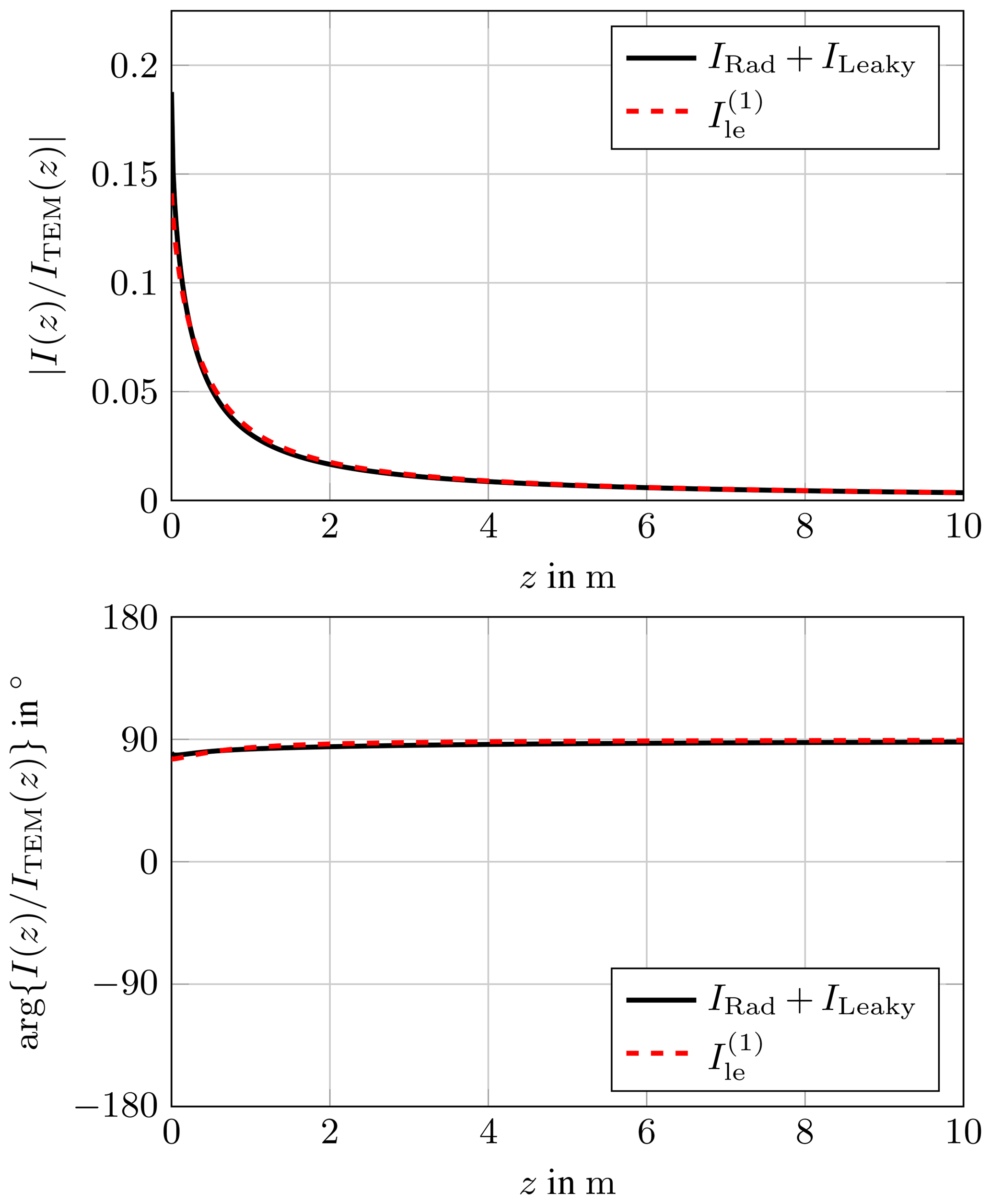
Figure 3 Comparison of the first iteration current with the leaky and radiation modes for $k=\mathrm{1}{\mathrm{m}}^{-\mathrm{1}}$, h=0.5 m, a=1 mm.

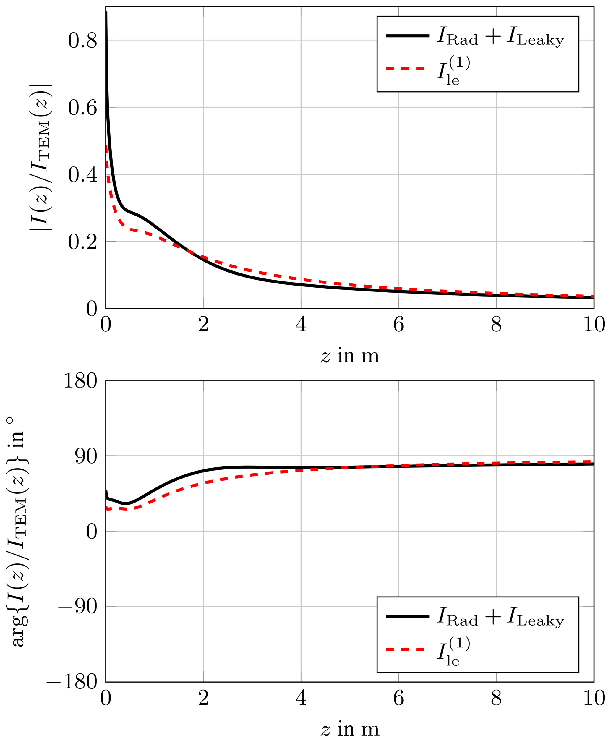
Figure 4 Comparison of the first iteration current with the leaky and radiation modes for $k=\mathrm{10}{\mathrm{m}}^{-\mathrm{1}}$, h=0.5 m, a=1 mm.

In Appendix A it is shown that the asymptotic expansion of the radiation mode and the first iteration coincide. Due to the exponential damping of the leaky modes, their asymptotic expansion is zero.

$$\begin{array}{}\text{(58)}& {\displaystyle }{I}_{\mathrm{le}}^{\left(\mathrm{1}\right)}\left(z\right)& {\displaystyle }\sim {\displaystyle \frac{V_{\mathrm{0}}}{\mathrm{2}{Z}_{\mathrm{C}}}}{\displaystyle \frac{\mathrm{4}\mathrm{j}k{h}^{\mathrm{2}}}{\mathrm{4}\ln \left(\frac{\mathrm{2}h}{a}\right)}}{\displaystyle \frac{\exp (-\mathrm{j}kz)}{z}}\text{(59)}& {\displaystyle }{I}_{\mathrm{Rad}}\left(z\right)& {\displaystyle }\sim {\displaystyle \frac{V_{\mathrm{0}}}{\mathrm{2}{Z}_{\mathrm{C}}}}{\displaystyle \frac{\mathrm{4}\mathrm{j}k{h}^{\mathrm{2}}}{\mathrm{4}\ln \left(\frac{\mathrm{2}h}{a}\right)}}{\displaystyle \frac{\exp (-\mathrm{j}kz)}{z}}\text{(60)}& {\displaystyle }{I}_{\mathrm{Leaky}}\left(z\right)& {\displaystyle }\sim \mathrm{0}\end{array}$$

This explains the improved accuracy of the approximation with increasing distance to the source.

It is interesting to note that the asymptotic approximation of the current of a semi infinite wire has the same form. It is derived in Weinstein (1969) using the Wiener-Hopf technique.

4.2 Plane Wave Excitation

The convergence of the iterative approach for the plane wave excitation is already illustrated in Rachidi and Tkachenko (2008).

It is notable that for θ→0 follows

$$\begin{array}{}\text{(61)}& {\displaystyle }\underset{\mathit{\theta }\to \mathrm{0}}{lim}{k}_{\mathit{\theta }}& {\displaystyle }=k\text{(62)}& {\displaystyle }\underset{\mathit{\theta }\to \mathrm{0}}{lim}G\left(k_{\mathit{\theta }}\right)& {\displaystyle }=G\left(k\right)=\mathrm{2}\ln \left({\displaystyle \frac{\mathrm{2}h}{a}}\right)\text{(63)}& {\displaystyle }\underset{\mathit{\theta }\to \mathrm{0}}{lim}{I}_{\mathrm{pw}}^{\left(\mathrm{0}\right)}\left(z\right)& {\displaystyle }={\displaystyle \frac{\mathrm{8}\mathit{\pi }}{\mathrm{2}\ln \left(\frac{\mathrm{2}h}{a}\right)}}\sqrt{{\displaystyle \frac{{\mathit{\epsilon }}_{\mathrm{0}}}{{\mathit{\mu }}_{\mathrm{0}}}}}\Vert {\mathit{E}}_{\mathrm{0}}\Vert h{\mathrm{e}}^{-\mathrm{j}kz}\text{(64)}& {\displaystyle }& {\displaystyle }={\displaystyle \frac{\mathrm{4}h\Vert {\mathit{E}}_{\mathrm{0}}\Vert }{\mathrm{2}{Z}_{\mathrm{C}}}}{\mathrm{e}}^{-\mathrm{j}kz}\text{(65)}& {\displaystyle }\underset{\mathit{\theta }\to \mathrm{0}}{lim}{I}_{\mathrm{pw}}^{\left(n\right)}\left(z\right)& {\displaystyle }=\mathrm{0}\end{array}$$

Hence, the iterative approach immediately converges to the exact solution when θ→0. Furthermore, the solution in Eq. (64) coincides with the TEM solution from the lumped excitation with an equivalent voltage $V_{\mathrm{0}}=\mathrm{4}h\Vert {\mathit{E}}_{\mathrm{0}}\Vert$. This equivalent behavior is already mentioned in Nitsch and Tkachenko (2002b).

5 Conclusions

The manuscript presents the exact and iterative solution for the current of an infinite wire above ground excited by a lumped and distributed source. The iterative approach approximates the system behavior independently of the excitation. It is shown that the iterative approach converges for reasonable wire dimensions. When there is a TEM mode present, it coincides with the zeroth iteration solution, which is know from classical transmission line theory. The first iteration, which can also be determined for arbitrary wires, approximates the radiation and leaky modes. They occur when a lumped disturbance, e. g. a lumped voltage source, is present on the wire.

Even though only an infinite wire was analyzed the results help to understand the propagation of currents along practical wires with discrete disturbances (lumped elements, sharp bend, … ). Furthermore, the manuscript presents another example where the iterative approach yields a very good approximation without much effort.

Appendix A: Asymptotic Expansion for the Radiation Mode and the First Iteration

The first iteration current is given in Eq. (57). As described in Abramowitz and Stegun (1972) the amplitude of the exponential integral E₁ vanishes for large arguments. For small arguments a series exists.

$$\begin{array}{ll}{\displaystyle }& {\displaystyle }{E}_{\mathrm{1}}\left(\mathrm{j}k\right(\sqrt{z^{\mathrm{2}}+a^{\mathrm{2}}}+\left|z\right|\left)\right)\\ \text{(A1)}& {\displaystyle }& {\displaystyle }-E_{\mathrm{1}}\left(\mathrm{j}k\right(\sqrt{z^{\mathrm{2}}+\mathrm{4}{h}^{\mathrm{2}}}+\left|z\right|\left)\right)\sim \mathrm{0}\text{(A2)}& {\displaystyle }& {\displaystyle }\sqrt{z^{\mathrm{2}}+a^{\mathrm{2}}}-\left|z\right|={\displaystyle \frac{a^{\mathrm{2}}}{\mathrm{2}\left|z\right|}}+\mathcal{O}\left(\right|z{|}^{-\mathrm{3}}){\displaystyle }& {\displaystyle }{E}_{\mathrm{1}}\left(\mathrm{j}k\right(\sqrt{z^{\mathrm{2}}+a^{\mathrm{2}}}-\left|z\right|\left)\right)=-\mathit{\gamma }-\ln \left({\displaystyle \frac{\mathrm{j}k{a}^{\mathrm{2}}}{\mathrm{2}\left|z\right|}}\right)\\ \text{(A3)}& {\displaystyle }& {\displaystyle }+\mathrm{j}k{\displaystyle \frac{a^{\mathrm{2}}}{\mathrm{2}\left|z\right|}}+\mathcal{O}\left(\right|z{|}^{-\mathrm{2}})\end{array}$$

where γ denotes the Euler-Mascheroni constant. Inserting the latter results into Eq. (57) yields

$$\begin{array}{ll}{\displaystyle }{I}_{\mathrm{le}}^{\left(\mathrm{1}\right)}\left(z\right)& {\displaystyle }\sim {\displaystyle \frac{V_{\mathrm{0}}}{\mathrm{2}{Z}_{\mathrm{C}}}}{\mathrm{e}}^{-\mathrm{j}k\left|z\right|}-{\displaystyle \frac{V_{\mathrm{0}}}{\mathrm{2}{Z}_{\mathrm{C}}}}{\displaystyle \frac{\mathrm{1}}{\mathrm{2}\ln \left(\frac{\mathrm{2}h}{a}\right)}}{\mathrm{e}}^{-\mathrm{j}k\left|z\right|}\\ \text{(A4)}& {\displaystyle }& {\displaystyle }\times \left[\mathrm{2}\ln \right({\displaystyle \frac{\mathrm{2}h}{a}})+\mathrm{j}k{\displaystyle \frac{a^{\mathrm{2}}-\mathrm{4}{h}^{\mathrm{2}}}{\mathrm{2}\left|z\right|}}]+\mathcal{O}\left(\right|z{|}^{-\mathrm{2}})\text{(A5)}& {\displaystyle }{I}_{\mathrm{le}}^{\left(\mathrm{1}\right)}\left(z\right)& {\displaystyle }\sim {\displaystyle \frac{V_{\mathrm{0}}}{\mathrm{2}{Z}_{\mathrm{C}}}}{\displaystyle \frac{\mathrm{j}k(\mathrm{4}{h}^{\mathrm{2}}-a^{\mathrm{2}})}{\mathrm{4}\ln \left(\frac{\mathrm{2}h}{a}\right)}}{\displaystyle \frac{\exp (-\mathrm{j}k|z\left|\right)}{\left|z\right|}}+\mathcal{O}\left(\right|z{|}^{-\mathrm{2}}).\end{array}$$

The radiation mode consists of an integral of the form

$$\begin{array}{}\text{(A6)}& J\left(z\right):=\underset{\mathrm{0}}{\overset{\mathrm{\infty }}{\int }}\mathrm{d}x{\mathrm{e}}^{-xz}f\left(x\right)\end{array}$$

with

$$\begin{array}{}\text{(A7)}& \begin{array}{rl}& f\left(x\right)={\displaystyle \frac{\mathrm{1}}{-x(x+\mathrm{2}\mathrm{j}k)}}\\ & \times [{\displaystyle \frac{\mathrm{1}}{K_{\mathrm{0}}(-a\sqrt{-x(x+\mathrm{2}\mathrm{j}k)})-K_{\mathrm{0}}(-\mathrm{2}h\sqrt{-x(x+\mathrm{2}\mathrm{j}k)})}}\\ & -{\displaystyle \frac{\mathrm{1}}{K_{\mathrm{0}}\left(a\sqrt{-x(x+\mathrm{2}\mathrm{j}k)}\right)-K_{\mathrm{0}}\left(\mathrm{2}h\sqrt{-x(x+\mathrm{2}\mathrm{j}k)}\right)}}]\end{array}\end{array}$$

The integral J(z) can be approximated for large z as described in Wong (2002). Due to the strong damping of the exponential function for large z

$$\begin{array}{}\text{(A8)}& {\displaystyle }J\left(z\right)& {\displaystyle }\sim \underset{\mathrm{0}}{\overset{\mathrm{\infty }}{\int }}\mathrm{d}x{\mathrm{e}}^{-xz}f\left(\mathrm{0}\right)\text{(A9)}& {\displaystyle }& {\displaystyle }={\displaystyle \frac{f\left(\mathrm{0}\right)}{z}}.\end{array}$$

After some lengthy but straight forward mathematical manipulation it can be shown that

$$\begin{array}{}\text{(A10)}& \underset{x\to \mathrm{0}}{lim}f\left(x\right)=-{\displaystyle \frac{\mathit{\pi }\mathrm{j}(\mathrm{4}{h}^{\mathrm{2}}-a^{\mathrm{2}})}{\left[\mathrm{2}\ln \right(\frac{\mathrm{2}h}{a}){]}^{\mathrm{2}}}}.\end{array}$$

Inserting the latter results into Eq. (27) yields

$$\begin{array}{}\text{(A11)}& {\displaystyle }{I}_{\mathrm{Rad}}\left(z\right)& {\displaystyle }\sim {\displaystyle \frac{\mathit{\pi }\mathrm{j}k(\mathrm{4}{h}^{\mathrm{2}}-a^{\mathrm{2}})}{\left[\mathrm{2}\ln \right(\frac{\mathrm{2}h}{a}){]}^{\mathrm{2}}}}{V}_{\mathrm{0}}\sqrt{{\displaystyle \frac{{\mathit{\epsilon }}_{\mathrm{0}}}{{\mathit{\mu }}_{\mathrm{0}}}}}{\displaystyle \frac{\exp (-\mathrm{j}kz)}{z}}\text{(A12)}& {\displaystyle }& {\displaystyle }={\displaystyle \frac{V_{\mathrm{0}}}{\mathrm{2}{Z}_{\mathrm{C}}}}{\displaystyle \frac{\mathrm{j}k(\mathrm{4}{h}^{\mathrm{2}}-a^{\mathrm{2}})}{\mathrm{4}\ln \left(\frac{\mathrm{2}h}{a}\right)}}{\displaystyle \frac{\exp (-\mathrm{j}kz)}{z}}.\end{array}$$

Appendix B: Parameter Study for the Convergence Condition

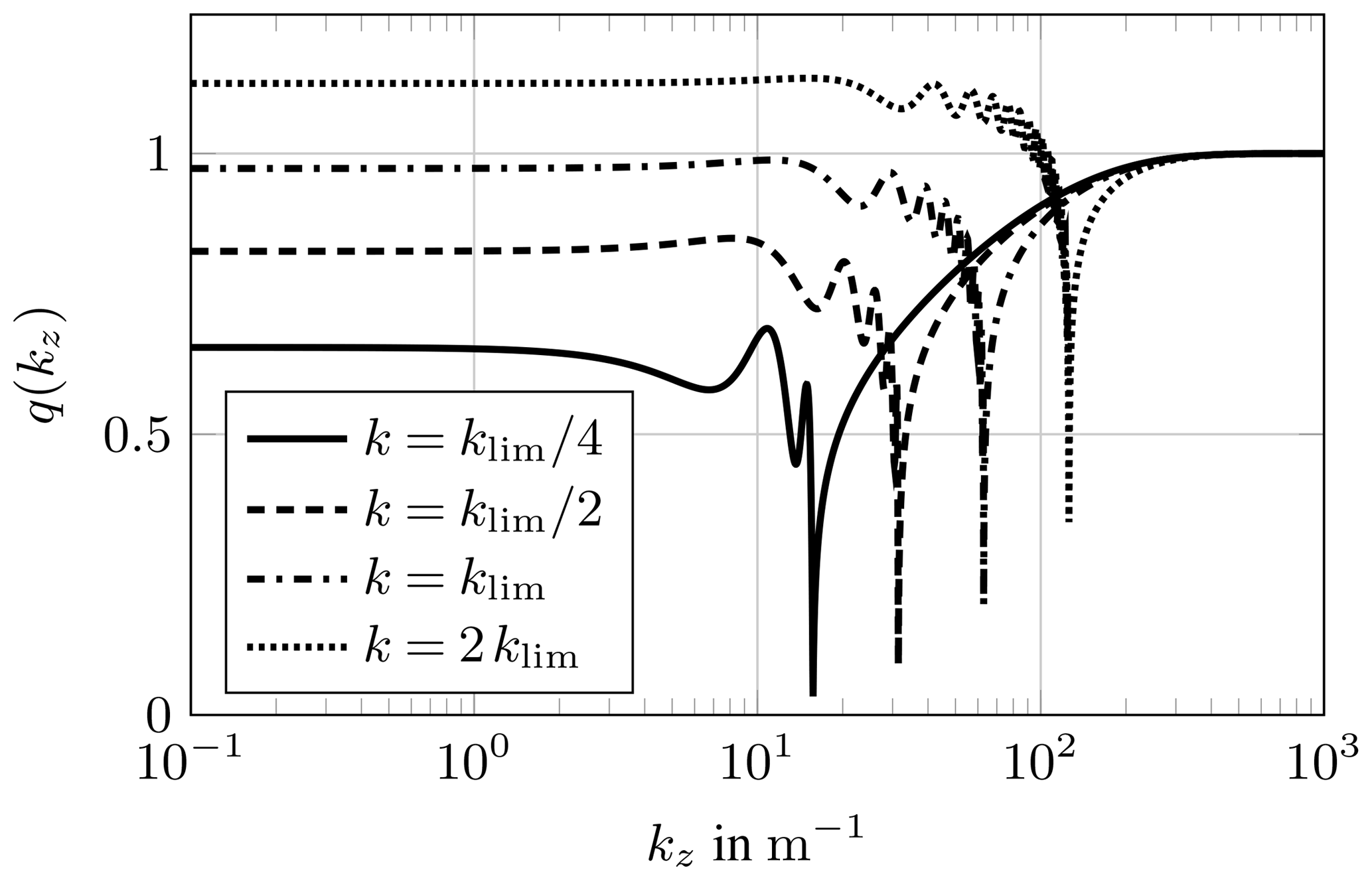
In the following some results of the parameter study are illustrated. As stated in Sect. 3 the function

$$\begin{array}{}\text{(B1)}& q\left(k_z\right)=|\mathrm{1}-{\displaystyle \frac{\stackrel{\mathrm{̃}}{G}\left(k_z\right)}{\mathrm{2}\ln \left(\frac{\mathrm{2}h}{a}\right)}}|\end{array}$$

needs to be smaller than 1 for the iterative approach to be convergent.

Figure B1 shows the function q(k_z) for different k. It can be seen that the convergence condition Eq. (39) holds as long as k≤k_lim. The upper bound k_lim is chosen such that $a<\mathit{\lambda }/\mathrm{10}$, where λ denotes the wavelength. This results in

$$\begin{array}{}\text{(B2)}& k_{\lim }={\displaystyle \frac{\mathrm{2}\mathit{\pi }}{\mathrm{10}a}}.\end{array}$$

If k increases, the thin wire approximation is not valid anymore, q(k_z) is larger than 1 for some k_z and the iterative approach diverges.

A lengthy but straight forward analytic analysis shows that q(k_z) is always smaller than 1 for all k_z>k.

Figure B1 Convergence condition for different frequencies k with h=0.5 m and a=10 mm.