Singularity Expansion Method for thin wires and the Method of Modal Parameters

Here, we describe a technique to define the Singularity Expansion Method (SEM) poles for short-circuited thin-wire structures developed using the Method of Modal Parameters (MoMP). The MoMP method consists of in the expansion of the system of mixed-potential integral equations (MPIE) into the Fourier series, including the kernels containing Green's function. Corresponding equations for Fourier modes contain infinite matrices of p.u.l. inductance and capacitance, and the solution for current can be obtained using the infinity matrix of p.u.l. impedance. The SEM poles are given by the zeros of the determinant of this matrix. For the case of the symmetrical circular loop, this equation transforms to one well-know from the literature. Numerical investigation of solutions for the poles of the first layer has shown good agreement with previously obtained analytical and numerical results for different wire configurations.

1 Introduction

Thin-wire transmission lines play an important role in EMC. Thin-wire transmission lines facilitate the transmission of the desired signals between electronic devices of different kinds. On the other hand, they are subject to different kinds of electronic interferences. Induced voltages are often the cause of the failure of electronic devices. Different numerical methods (e.g., MoM, FDTD) can be applied to calculate induced currents and voltages, but these are not very helpful for gaining insight into the physics of coupling phenomena (e.g., to make a qualitative analysis of the system response for various values of system parameters, including the case of a statistically defined system or field parameters).

In contrast, the Singularity Expansion Method (SEM) (see pioneer paper Baum, 1971, and reviews of results in books Baum et al., 2012; Tesche et al., 1997) represents the scattering object as a set of oscillators, in which complex frequencies are poles of the response function, which do not depend on the type of excitation of the system. This set of poles yield the main contribution to the coupling response of the object, both in the frequency and time domains. It also defines the radiation of the system and the scattering amplitude. Moreover, the SEM poles can be used for the identification of the systems. Recently, this method has attracted increasing interest in connection to the problem of target identification (Myers et al., 2011a, b; Giri and Tesche, 2012). However, the main method for obtaining the SEM expansion for a general system is the processing of numerical (e.g., Method of Moments) data (Senior and Pond, 1981; Singaraju et al., 1976).

On the other hand, the application of SEM to thin-wire systems (antennas and transmission lines) has several specific features that simplify the investigation of the SEM expansion, especially when the analytic form of the response function is known. Such response functions were investigated earlier for the straight transmission lines, when the length of the line is essentially larger relative to its height (Tkachenko et al., 2013, 2014, 2016; Middelstaedt et al., 2016, 2018). To do this, the so-called asymptotic approach was used (Tkachenko et al., 2001; Rachidi and Tkachenko, 2008). However, the application of the asymptotic approach is restricted by long straight lines. In the present work, we describe the application of another analytical method, the method of modal parameters (Nitsch and Tkachenko, 2005, 2007) for the investigation of the SEM poles. This analytical technique can be applied for thin wires of arbitrary geometrical form and arbitrary excitations.

The rest of the paper is organized in the following. In Sect. 2, the method of modal parameters will be briefly described. In Sect. 3, we present the analytical approach and a numerical algorithm for finding the SEM poles. In Sect. 4, some numerical results and comparisons with other methods will be described. Section 5 concludes the paper.

2 Method of Modal Parameters for finite wires

We consider a wire of arbitrary geometrical form above a perfect-conducting ground (Fig. 1). The wire is represented by a three-dimensional space curve r(l) parameterized with its natural parameter $l(\mathrm{0}\le l\le L/\mathrm{2}$, where L∕2 is the length of the wire). It is assumed that both terminals of the line are connected with the ground. The wire is thin, i.e. the radius of the wire is essentially smaller relative to all other characteristic dimensions of the problem (e.g., wavelength λ, length of the line L∕2). The line is excited by an arbitrary electromagnetic field, which can be external (e.g., an exciting plane wave) or a lumped voltage source (a load also can be consider as a current controlled voltage source). Since the thin-wire approximation is used, it is assumed that: the azimuthal component of the current is neglected; the charge density and the current are concentrated on the wire axis; and the boundary condition for the tangential component of the electric field is satisfied on the surface of the wire. The current I(l^′) and potential ϕ(l) along the wire are described by the integrodifferential Mixed Potential Integral Equations (MPIE, e.g., Nitsch and Tkachenko, 2007). Usually, the system of MPIE is defined on the “physical” wire in the upper half-plane when the perfectly conducting ground is taking into account by mirroring the corresponding Green's functions. Another way is to add to a physical wire its mirror reflection and to consider the loop closed and completed (Fig. 2). During this procedure, the ground plane is removed. To excite only those modes, as in the initial problem, one has to also to consider a symmetrical external and lumped excitation. Such a procedure yields the MPIE system for the closed loop:

$$\begin{array}{}\text{(1a)}& {\displaystyle }\left\{\begin{array}{l}\frac{\mathrm{d}\mathit{\varphi }\left(l\right)}{\mathrm{d}l}+j\mathit{\omega }\frac{{\mathit{\mu }}_{\mathrm{0}}}{\mathrm{4}\mathit{\pi }}\underset{\mathit{\left\{}L\mathit{\right\}}}{\oint }{\mathit{e}}_l\left(l\right)\cdot {\mathit{e}}_l\left(l^{\prime }\right)g(l,l^{\prime })I\left(l^{\prime }\right)\mathrm{d}{l}^{\prime }=E_l^{\mathrm{ex}}\left(l\right)\\ \underset{\mathit{\left\{}L\mathit{\right\}}}{\oint }g(l,l^{\prime })\frac{\mathrm{d}I\left(l^{\prime }\right)}{\mathrm{d}{l}^{\prime }}\mathrm{d}{l}^{\prime }+j\mathit{\omega }\mathrm{4}\mathit{\pi }{\mathit{\epsilon }}_{\mathrm{0}}\mathit{\varphi }\left(l\right)=\mathrm{0}\end{array}\right.;\text{(1b)}& {\displaystyle }{\mathit{e}}_l\left(l\right):=\partial \mathit{r}\left(l\right)/\partial l,\left|{\mathit{e}}_l\left(l\right)\right|=\mathrm{1};\text{(1c)}& {\displaystyle }g(l,l^{\prime })={\displaystyle \frac{e^{-jk\sqrt{{\left(\mathit{r}\left(l\right)-\mathit{r}\left(l^{\prime }\right)\right)}^{\mathrm{2}}+r_{\mathrm{0}}^{\mathrm{2}}}}}{\sqrt{{\left(\mathit{r}\left(l\right)-\mathit{r}\left(l^{\prime }\right)\right)}^{\mathrm{2}}+r_{\mathrm{0}}^{\mathrm{2}}}}}\end{array}$$

Here L is the length of the complete wire loop, $E_l^{\mathrm{ex}}\left(l\right)$ is a tangential component of a symmetrized exciting field, e_l(l) is a tangential unit vector, and $g(l,l^{\prime })$ is a scalar Green's function defined on the curved wire.

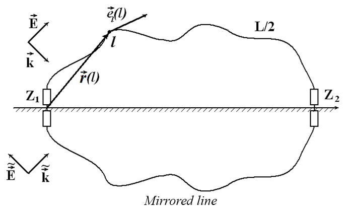
Figure 1 Inhomogeneous thin conductor over a conductive ground excited by external field and lumped source.

Figure 2 Short-circuited, semi-circular wire.

All functions of the natural parameter l in Eqs. (1a)–(1c) are periodical, i.e., $\mathit{r}(l+L)=\mathit{r}\left(l\right)$ and they can be expanded in a complete orthogonal set of functions exp (−jk_ml) with $k_m:=\frac{\mathrm{2}\mathit{\pi }m}{L},m=\mathrm{\dots }-\mathrm{1},\mathrm{0},\mathrm{1}\mathrm{\dots }$ They can be represented in the form

$$\begin{array}{}\text{(2a)}& {\displaystyle }{E}_l^{\mathrm{ex}}\left(l\right)=\sum _{m=-\mathrm{\infty }}^{\mathrm{\infty }}{E}_{l,m}^{\mathrm{ex}}{e}^{-j{k}_{m}l}=[e^{-j{k}_{m}l}{]}^T\cdot {\mathit{E}}_l^{\mathrm{ex}};\text{(2b)}& {\displaystyle }\mathit{\varphi }\left(l\right)=\sum _{m=-\mathrm{\infty }}^{\mathrm{\infty }}{\mathit{\varphi }}_m{e}^{-j{k}_{m}l}=[e^{-j{k}_{m}l}{]}^T\cdot \mathbf{\Phi };\text{(2c)}& {\displaystyle }I\left(l\right)=\sum _{m=-\mathrm{\infty }}^{\mathrm{\infty }}{I}_m{e}^{-j{k}_{m}l}=[e^{-j{k}_{m}l}{]}^T\cdot \mathit{I}\end{array}$$

Here ${\mathit{E}}_l^{\mathrm{ex}}$, Φ and I are column vectors of the Fourier coefficients of the exciting electric field, potential, and current; and $\left[e^{-j{k}_{m}l}\right]:=[\mathrm{\dots }{e}^{-j{k}_{-\mathrm{1}}l},\mathrm{1},e^{j{k}_{\mathrm{1}}l},\mathrm{\dots }{]}^T$ is an infinite column vector of basic orthogonal functions.

Then, the MPIE system (Eq. 1a) can be re-written in a modal representation:

$$\begin{array}{}\text{(3a)}& {\displaystyle }\left\{\begin{array}{c}-j\mathit{k}\cdot \mathbf{\Phi }+j\mathit{\omega }{\mathit{L}}^{\prime }\cdot \mathit{I}={\mathit{E}}_l^{\mathrm{ex}}\\ -j\mathit{k}\cdot \mathit{I}+j\mathit{\omega }{\mathit{C}}^{\prime }\cdot \mathbf{\Phi }=\mathrm{0}\end{array}\right.;\text{(3b)}& {\displaystyle }\mathit{k}=\mathrm{diag}\left(k_m\right);\text{(3c)}& {\displaystyle }{\mathit{L}}^{\prime }={\displaystyle \frac{{\mathit{\mu }}_{\mathrm{0}}}{\mathrm{2}\mathit{\pi }}}{\mathbf{G}}_L;\text{(3d)}& {\displaystyle }{\mathit{C}}^{\prime }={\displaystyle \frac{{\mathit{\mu }}_{\mathrm{0}}}{\mathrm{2}\mathit{\pi }}}\mathrm{2}\mathit{\pi }{\mathit{\epsilon }}_{\mathrm{0}}{\mathbf{G}}_C^{-\mathrm{1}}\end{array}$$

where we introduce infinite square matrixes of inductance per-unit-length L^′ and capacitance per-unit-length C^′, which can be obtained by expansion of the kernels of the system (Eq. 1a) in a double Fourier series:

$$\begin{array}{}\text{(4)}& {\displaystyle }\begin{array}{rl}{\mathbf{G}}_L& =\left[G_{m_{\mathrm{1}},m_{\mathrm{2}}}^L\right];\\ G_{m_{\mathrm{1}},m_{\mathrm{2}}}^L& =\underset{\mathit{\left\{}L\mathit{\right\}}}{\oint }\mathrm{d}{l}_{\mathrm{1}}\underset{\mathit{\left\{}L\mathit{\right\}}}{\oint }\mathrm{d}{l}_{\mathrm{2}}{\mathit{e}}_l\left(l_{\mathrm{1}}\right)\cdot {\mathit{e}}_l\left(l_{\mathrm{2}}\right)g(l_{\mathrm{1}},l_{\mathrm{2}})\\ & \cdot \exp (-j{k}_{m_{\mathrm{2}}}{l}_{\mathrm{2}}+j{k}_{m_{\mathrm{1}}}{l}_{\mathrm{1}})\end{array}\text{(5)}& {\displaystyle }\begin{array}{rl}{\mathbf{G}}_C& =\left[G_{m_{\mathrm{1}},m_{\mathrm{2}}}^C\right];\\ G_{m_{\mathrm{1}},m_{\mathrm{2}}}^C& =\underset{\mathit{\left\{}L\mathit{\right\}}}{\oint }\mathrm{d}{l}_{\mathrm{1}}\underset{\mathit{\left\{}L\mathit{\right\}}}{\oint }\mathrm{d}{l}_{\mathrm{2}}g(l_{\mathrm{1}},l_{\mathrm{2}})\exp (-j{k}_{m_{\mathrm{2}}}{l}_{\mathrm{2}}+j{k}_{m_{\mathrm{1}}}{l}_{\mathrm{1}})\end{array}\end{array}$$

Using the modal representation of MPIE (Eq. 3a) one can easily obtain a formal solution for the column-vectors of the current and potential (Eq. 6), where Z^′ is an infinite modal impedance per-unit-length matrix (Eq. 7a), which defines the scattering field on

$$\begin{array}{}\text{(6)}& \left\{\begin{array}{l}\mathit{I}={\mathbf{Z}}^{-\mathrm{1}}\cdot {\mathit{E}}_l^{\mathrm{ex}}\\ \mathbf{\Phi }=\frac{\mathrm{1}}{j\mathit{\omega }}{\mathit{C}}^{-\mathrm{1}}\cdot j\mathit{k}\cdot {\mathbf{Z}}^{-\mathrm{1}}\cdot {\mathit{E}}_l^{\mathrm{ex}}\end{array}\right.;\end{array}$$

$$\begin{array}{}\text{(7a)}& {\displaystyle }\begin{array}{rl}{\mathbf{Z}}^{\prime }\left(j\mathit{\omega }\right):& ={\displaystyle \frac{\mathit{k}\cdot {{\mathit{C}}^{\prime }}^{-\mathrm{1}}\cdot \mathit{k}}{j\mathit{\omega }}}+j\mathit{\omega }{\mathit{L}}^{\prime }\\ & ={\displaystyle \frac{{\mathit{\eta }}_{\mathrm{0}}}{\mathrm{4}\mathit{\pi }jk}}\left[\mathit{k}\cdot {\mathbf{G}}_C\cdot \mathit{k}-k^{\mathrm{2}}{\mathbf{G}}_L\right];\end{array}\text{(7b)}& {\displaystyle }{\mathit{E}}_l^{\mathrm{sc}}=-{\mathbf{Z}}^{\prime }\cdot \mathit{I};\text{(7c)}& {\displaystyle }\stackrel{\mathrm{‾}}{W}={\displaystyle \frac{L}{\mathrm{4}}}Re\left\{{\mathit{I}}^{+}\cdot \mathbf{Z}\cdot \mathit{I}\right\};\end{array}$$

the boundary of the wire (Eq. 7b) and the radiation of the system (Eq. 7c) (Nitsch and Tkachenko, 2007).

The general solution (Eq. 6) is valid for any exciting field, including a plane wave excitation (Krauthauser et al., 2005) or lumped voltage sources (Nitsch and Tkachenko, 2005, 2007; Tkachenko et al., 2011). Moreover, lumped loads can be considered using current-controlled sources with unknown current amplitudes, which can be defined by solution of system of linear equations.

In this paper, however, we restrict our scope to the case of a short-circuited wire with an arbitrary excitation.

For the case of the semi-circular wire (when the closed wire is a circular loop, a structure with high symmetry with constant curvature $\mathit{K}=\mathrm{1}/R=\mathrm{const}$ and zero torsion T=0), the modal inductance, capacitance and impedance per-unit-length are diagonal matrices and one can obtain a known solution for the induced current in the thin-wire approximation (Wu, 1962)

$$\begin{array}{}\text{(8a)}& {\displaystyle }{L}_{m_{\mathrm{1}},m_{\mathrm{2}}}^{\prime }=L_{m_{\mathrm{1}}}^{\prime }{\mathit{\delta }}_{m_{\mathrm{1}},m_{\mathrm{2}}};\text{(8b)}& {\displaystyle }{L}_m^{\prime }={\mathit{\mu }}_{\mathrm{0}}R{\displaystyle \frac{g_{m+\mathrm{1}}+g_{m-\mathrm{1}}}{\mathrm{4}}};\text{(8c)}& {\displaystyle }{C}_{m_{\mathrm{1}},m_{\mathrm{2}}}=C_{m_{\mathrm{1}}}\cdot {\mathit{\delta }}_{m_{\mathrm{1}},m_{\mathrm{2}}};\text{(8d)}& {\displaystyle }{C}_m={\displaystyle \frac{\mathrm{2}{\mathit{\epsilon }}_{\mathrm{0}}}{R{g}_m}}\end{array}$$

$$\begin{array}{}\text{(9a)}& {\displaystyle }{Z}_{m_{\mathrm{1}},m_{\mathrm{2}}}^{\prime }\left(j\mathit{\omega }\right)=Z_{m_{\mathrm{1}}}^{\prime }\left(j\mathit{\omega }\right)\cdot {\mathit{\delta }}_{m_{\mathrm{1}},m_{\mathrm{2}}};\text{(9b)}& {\displaystyle }{Z}_m^{\prime }\left(j\mathit{\omega }\right)=j\mathit{\omega }{L}_m+{\displaystyle \frac{k_m^{\mathrm{2}}}{j\mathit{\omega }{C}_m}};\text{(9c)}& {\displaystyle }{k}_m:={\displaystyle \frac{m}{R}},m=\mathrm{\dots }-\mathrm{1},\mathrm{0},\mathrm{1}\mathrm{\dots }\end{array}$$

where

$$\begin{array}{}\text{(10)}& g_m=\underset{\mathrm{0}}{\overset{\mathrm{2}\mathit{\pi }R}{\int }}{\displaystyle \frac{e^{j{k}_{m}l-jk\sqrt{\mathrm{4}{R}^{\mathrm{2}}{\sin }^{\mathrm{2}}(l/\mathrm{2}R)+a^{\mathrm{2}}}}}{\sqrt{\mathrm{4}{R}^{\mathrm{2}}{\sin }^{\mathrm{2}}(l/\mathrm{2}R)+r_{\mathrm{0}}^{\mathrm{2}}}}}\mathrm{d}l\end{array}$$

3 SEM poles and Method of Modal Parameters

According to the definition of the SEM poles they are natural frequencies of the system, i.e., “complex frequencies at which an integral equation representation of the scattering problem has solution with no incident electromagnetic field” (Baum). In the initial papers, “they can be found from the zeros of the determinant of the corresponding moment method matrixes” (Baum). Now, however, the MPIE system is represented in the modal form. Therefore, the SEM poles can also be found from the zeros of the determinant of the impedance per-unit length matrix (Eqs. 11a, b).

$$\begin{array}{}\text{(11a)}& {\displaystyle }\det \left({\mathbf{Z}}^{\prime }\right(j\mathit{\omega }\left)\right)=\mathrm{0}\mathrm{or}\text{(11b)}& {\displaystyle }\det [k^{\mathrm{2}}\mathbf{1}-{\mathbf{G}}_L^{-\mathrm{1}}(k)\cdot \mathit{k}\cdot {\mathbf{G}}_C(k)\cdot \mathit{k}]=\mathrm{0}\end{array}$$

For the symmetrical circular loop (Eqs. 11a, b) splits and one has separate simple equations (Eq. 11b) for each integer m.

$$\begin{array}{}\text{(12a)}& {\displaystyle }\det \left(Z_m\right(j\mathit{\omega }\left)\right)=\mathrm{0}\mathrm{or}\text{(12b)}& {\displaystyle }{k}^{\mathrm{2}}-{\displaystyle \frac{\mathrm{2}{k}_m^{\mathrm{2}}{g}_m\left(k\right)}{g_{m+\mathrm{1}}\left(k\right)+g_{m-\mathrm{1}}\left(k\right)}}=\mathrm{0};\end{array}$$

The equation for the poles (Eq. 12b) up to notation coincides with the one used by Blackburn (1976) and Blackburn and Wilton (1978), if one assumes thin-wire approximation. In these works, detailed research of the poles for circular loop, including the case of high layers, was carried out.

It is noteworthy that from Eqs. (6), (7a), and (11a), the SEM poles are independent of the kind of excitation of the system (e.g., distributed excitation, lumped excitation). Below we describe both an approximate analytical method and a numerical algorithm to find the poles.

3.1 Analytic approach: perturbation theory for SEM poles

It is possible to show that for the case of infinitely thin wire r₀→0, the matrices G_L and G_C become diagonal and approximately equal to each other (${\mathbf{G}}_L\approx {\mathbf{G}}_C\approx \mathrm{2}\ln (\stackrel{\mathrm{̃}}{L}/r_{\mathrm{0}})\cdot \mathbf{1}$, where $\stackrel{\mathrm{̃}}{L}$ is some length parameter of the system, (i.e., for the circle $\stackrel{\mathrm{̃}}{L}\approx \mathrm{2}R)$, which leads to ${\mathbf{G}}_L^{-\mathrm{1}}\left(k\right)\cdot \mathit{k}\cdot {\mathbf{G}}_C\left(k\right)\cdot \mathit{k}\to {\mathit{k}}^{\mathrm{2}}$. Thus, we can obtain the approximate equation for the SEM - poles, which has a simple solution:

$$\begin{array}{}\text{(13)}& \begin{array}{rl}{k}^{\mathrm{2}}& \cdot \mathbf{1}-{\mathit{k}}^{\mathrm{2}}=\mathrm{0}\Rightarrow k^{\mathrm{2}}=k_m^{\mathrm{2}}\\ & \Rightarrow k_m^{\left(\mathrm{0}\right)}=\pm \mathrm{2}\mathit{\pi }m/L,m=\mathrm{\dots }-\mathrm{2},-\mathrm{1},\mathrm{0},\mathrm{1},\mathrm{2}\mathrm{\dots }\end{array}\end{array}$$

These values can be used as a zero-order approximation of the iteration (perturbation theory) solution. Any subsequent iteration can be evaluated from the previous iteration as:

$$\begin{array}{}\text{(14)}& \begin{array}{rl}\det & \left[\mathrm{diag}\right((k_m^{(n+\mathrm{1})}{)}^{\mathrm{2}}-{\mathbf{G}}_L^{-\mathrm{1}}(k_m^{\left(n\right)})\cdot \mathit{k}\\ & \cdot {\mathbf{G}}_C\left(k_m^{\left(n\right)}\right)\cdot \mathit{k}]=\mathrm{0},n=\mathrm{0},\mathrm{1},\mathrm{2},\mathrm{\dots }\end{array}\end{array}$$

In particular, for the circle wire, the solution of this equation is:

$$\begin{array}{}\text{(15)}& \begin{array}{rl}{k}_m^{(n+\mathrm{1})}& =k_m^{\left(n\right)}\sqrt{{\displaystyle \frac{\mathrm{2}{g}_m\left(k_m^{\left(n\right)}\right)}{g_{m+\mathrm{1}}\left(k_m^{\left(n\right)}\right)+g_{m-\mathrm{1}}\left(k_m^{\left(n\right)}\right)}}},\\ & n=\mathrm{0},\mathrm{1},\mathrm{2},\mathrm{\dots };k_m^{\left(\mathrm{0}\right)}=k_m=m/R\end{array}\end{array}$$

Note that, as in the case of the circle wire, the SEM poles in the general case can be classified under the index m, which defines the number of waves of current along the thin wire. The considered iteration solution yields the poles of the so-called first layer, which are nearest to the real axis.

3.2 Numerical realization of the Method of Modal Parameters – algorithm of solution equation for the SEM poles

In this sub-section we describe the numerical realization of the method of modal parameters. For the first step, it is necessary to calculate the matrix elements of the capacity-like and inductivity-like G-matrixes (Eqs. 4–5). This is realized by double numerical integration. The first integral is solved numerically using the trapezoidal rule with 10 000 points. An important circumstance here is that the first integration is carrying out with function $g(l,l^{\prime })$, which has a “singularity” with characteristic dimension r₀, when $l\approx l^{\prime }$. Therefore, a step of the first integration Δ must describe the singularity of the Green's function: in other words, there must be several points of integration on the radius of the wire (e.g., if the complete length of the loop L is about 20 m, and the radius of the wire is r₀=1 cm, we have Δ = 20/10 000 = 2 mm, i.e., $a/\mathrm{\Delta }=\mathrm{5}$). However, the second integration contains a smooth integrand obtained as a result of the first integration, where the characteristic length is about the wavelength or length of non-uniformity of the wire. Tests have shown that 500 intervals are enough for the second integration. Of course, in numerical calculations, we use the finite matrix instead of the infinite matrix. The calculations show that, if we consider a matrix with order $M_{max}(-M_{max},-M_{max}+\mathrm{1},\mathrm{\dots }\mathrm{0}\mathrm{\dots }{M}_{max}-\mathrm{1},M_{max}$, i.e., with $(\mathrm{2}{M}_{max}+\mathrm{1})\times (\mathrm{2}{M}_{max}+\mathrm{1})$ elements), it issufficient to define the SEM poles for index m up to $M_{max}-\mathrm{2}$.

The knowledge of the matrices G_L and G_C gives a possibility to define a matrix Z^′. Up to the constant factor this matrix is given by:

$$\begin{array}{}\text{(16)}& {\mathbf{Z}}^{\prime }\sim k^{\mathrm{2}}\cdot {\mathbf{G}}_L\left(k\right)-\mathit{k}\cdot {\mathbf{G}}_C\left(k\right)\cdot \mathit{k}\end{array}$$

Next, the determinant of Z^′(x) is defined as a function of a normalized complex wave number $x:=k\cdot L/\mathrm{2}\mathit{\pi }$. Then, we look for the solution using the Newton algorithm. As the zero-order approximation for the SEM poles of the first layer for the wiring structure short-circuited at both ends, the next values are used (see Eq. 13)

$$\begin{array}{}\text{(17)}& x_m^{\left(\mathrm{0}\right)}=m\end{array}$$

Then we begin an iteration procedure. Because the calculation of the double integrals for all ($\mathrm{2}{M}_{max}+\mathrm{1}\times \mathrm{2}{M}_{max}+\mathrm{1}$) matrix elements requires a long time (about 30 min on a HP ENVY 17 Notebook personal computer with processor Intel(R) Core(TM) i7-550U CPU@240 GHz using the Fortran code), we will do this for the function:

$$\begin{array}{}\text{(18)}& \begin{array}{rl}F(\stackrel{\mathrm{̃}}{x},x)& :=\det \left({\stackrel{\mathrm{̃}}{k}}^{\mathrm{2}}\cdot {\mathbf{G}}_L\left(k\right)-\mathit{k}\cdot {\mathbf{G}}_C\left(k\right)\cdot \mathit{k}\right)\\ & \mathrm{where}x:=k\cdot L/\mathrm{2}\mathit{\pi },\stackrel{\mathrm{̃}}{x}:=\stackrel{\mathrm{̃}}{k}\cdot L/\mathrm{2}\mathit{\pi }\end{array}\end{array}$$

The iterations are carried out in two circles. In the internal circle (15 iterations), we use the Newton algorithm only for the value $\stackrel{\mathrm{̃}}{x}$ for a fixed value x

$$\begin{array}{}\text{(19)}& \begin{array}{rl}{\stackrel{\mathrm{̃}}{x}}_m^{\left(j\right)}& :={\stackrel{\mathrm{̃}}{x}}_m^{(j-\mathrm{1})}-{\displaystyle \frac{F({\stackrel{\mathrm{̃}}{x}}_m^{(j-\mathrm{1})},x_m^{\left(i\right)})}{{\left.\frac{\partial }{\partial \stackrel{\mathrm{̃}}{x}}F(\stackrel{\mathrm{̃}}{x},x_m^{\left(i\right)})\right|}_{\stackrel{\mathrm{̃}}{x}={\stackrel{\mathrm{̃}}{x}}_m^{(j-\mathrm{1})}}}},\\ & j=\mathrm{1}\mathrm{\dots }{J}_{max}=\mathrm{15}\end{array}\end{array}$$

For the next external circle, we repeat this procedure for the $x_m^{(i+\mathrm{1})}=x_m^{\left(I_{max}\right)}$, repeating this procedure $I_{max}=\mathrm{3}$ times (i=0, 1, 2…3). Both initial values are the same $x_m^{\left(\mathrm{0}\right)}={\stackrel{\mathrm{̃}}{x}}_m^{\left(\mathrm{0}\right)}=m$.

4 Numerical results for the SEM poles

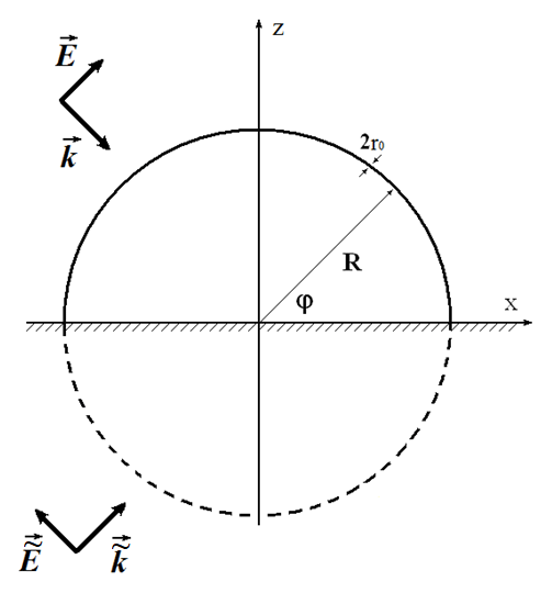
4.1 Short-circuited semi-circular wire

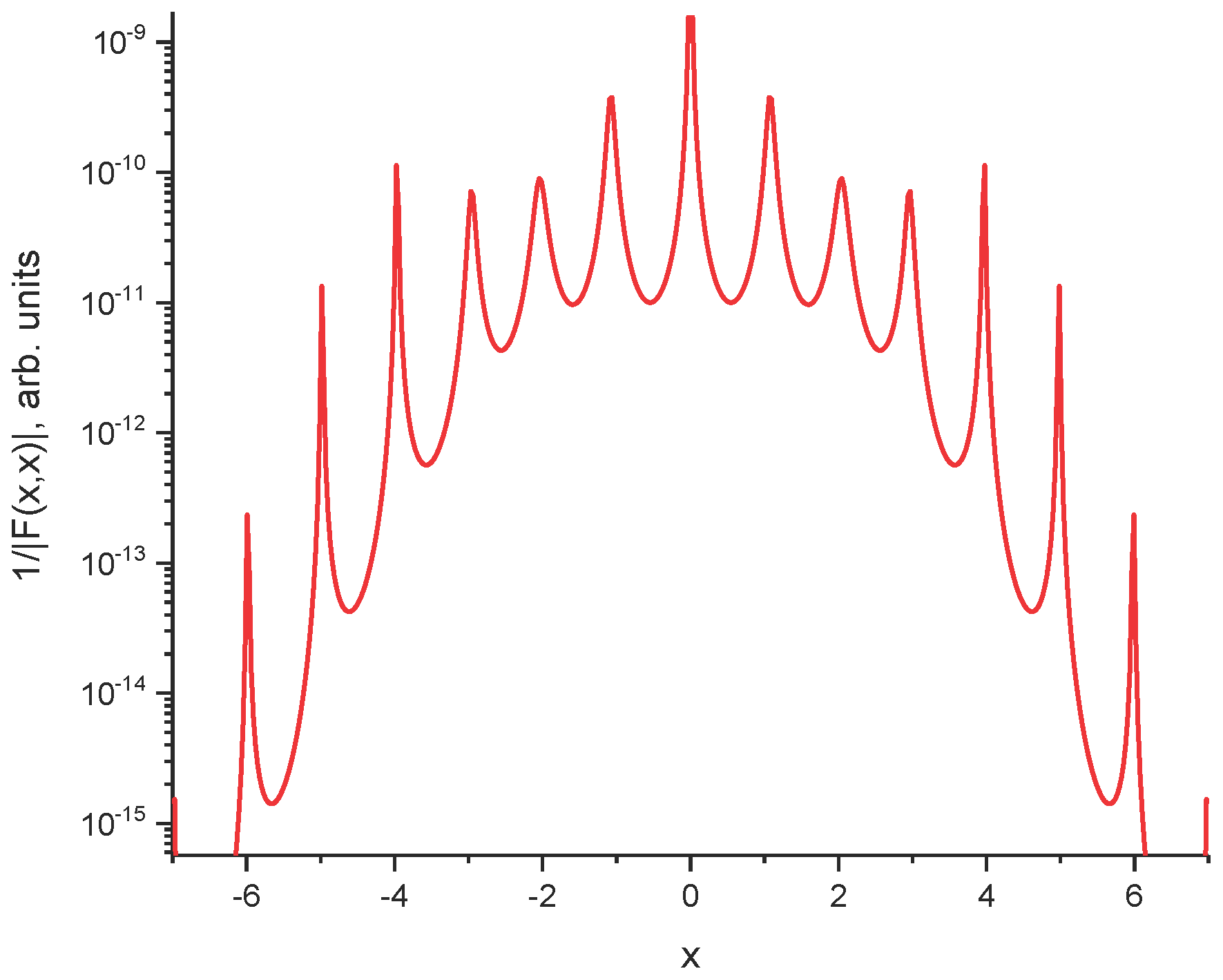
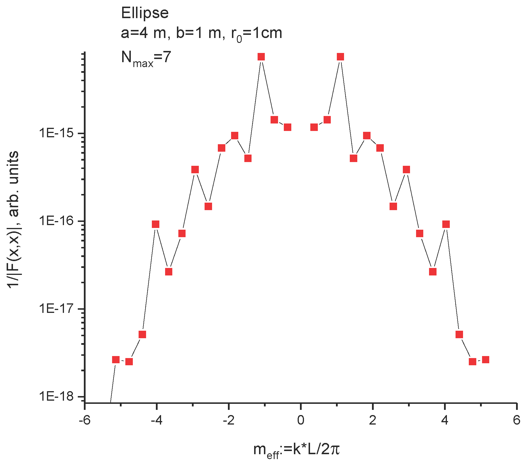
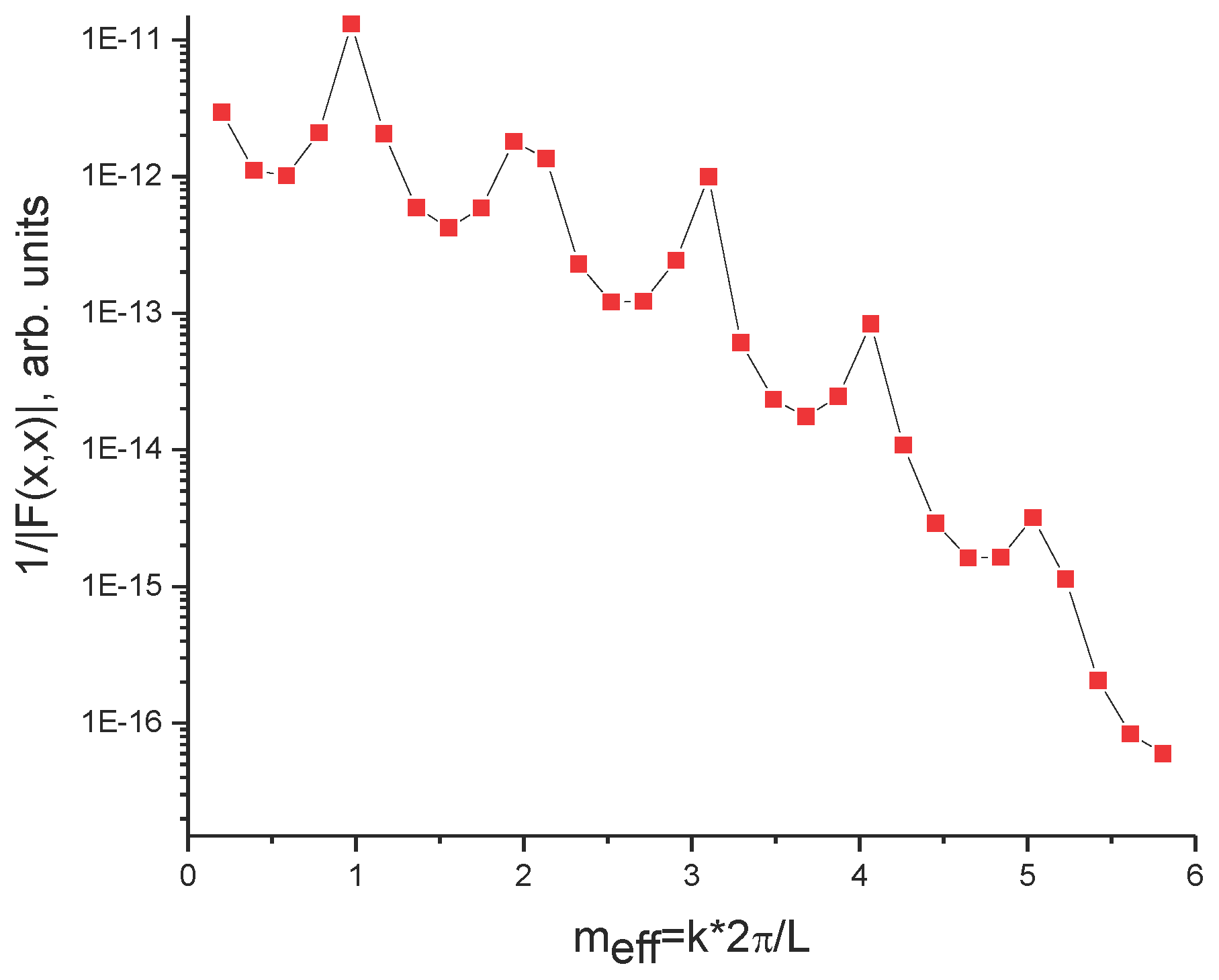
To check the method, we consider a vertical, short-circuited, semi-circular wire above a perfect conducting ground (Fig. 2). The parameters of the structure are: R=4 m and r₀=1 cm. The matrixes G_C(k) and G_L(k) are calculated by double integration and partially presented in Figs. 4–6. Using the exact calculations this matrix must be diagonal (see Eqs. 8–10). The relative value of the off-diagonal elements relative to diagonal elements represents the error of the method (about 10⁻³–10⁻⁴). But practically, the matrix Z^′ is diagonal and coincides with the exact result. The determinant of this matrix has minimum approximately for x≈m¹ (see Fig. 3 for the inverse value, which has maximums).

Figure 3 Function $\mathrm{1}/\left|F\right(x,x\left)\right|$ for the circular wire.

Figure 4 The real part of the matrix G_L for the circular wire. $k=\mathrm{2.3}/R$.

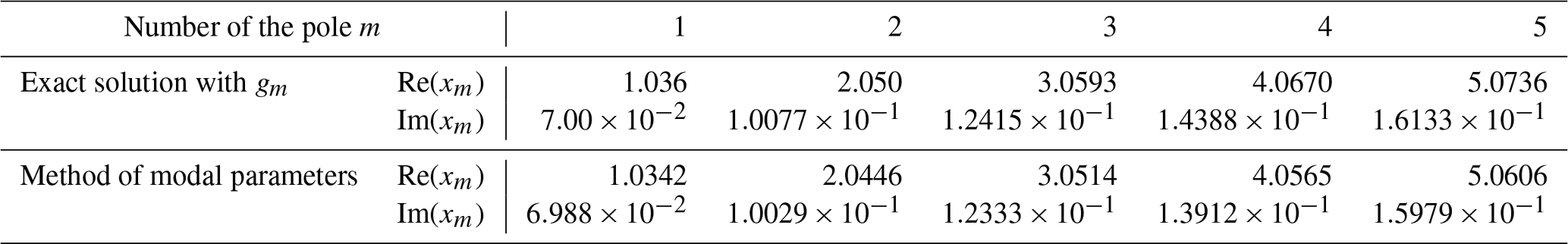
The comparison of the values of the poles of the first layer obtained using the numerical algorithm described above with the solution of the exact Eq. (12b) obtained by Maple software has shown excellent agreement (Table 1). Note that for corresponding values of the parameters of the circular loop the values of the SEM poles of the first layer obtained by the two methods described above coincide with these one obtained earlier by Umashankar and Wilton (1974).

Figure 5 The real part of the matrix G_C for the circular wire. $k=\mathrm{2.3}/R$.

Figure 6 The real part of the matrix Z^′ for the circular wire. $k=\mathrm{2.3}/R$.

Table 1 SEM poles of the first layer for the circular wire.

4.2 Short-circuited semi-elliptical wire

As the second example, we consider the semi-elliptical short-circuited wire above a perfectly conducting ground (Fig. 7).

Figure 7 Short-circuited semi-elliptical wire.

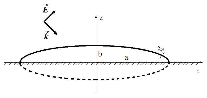
The parameters of the full ellipse (initial wire plus mirrored wire) are: a=4 m, b=1 m, r₀=1 cm.

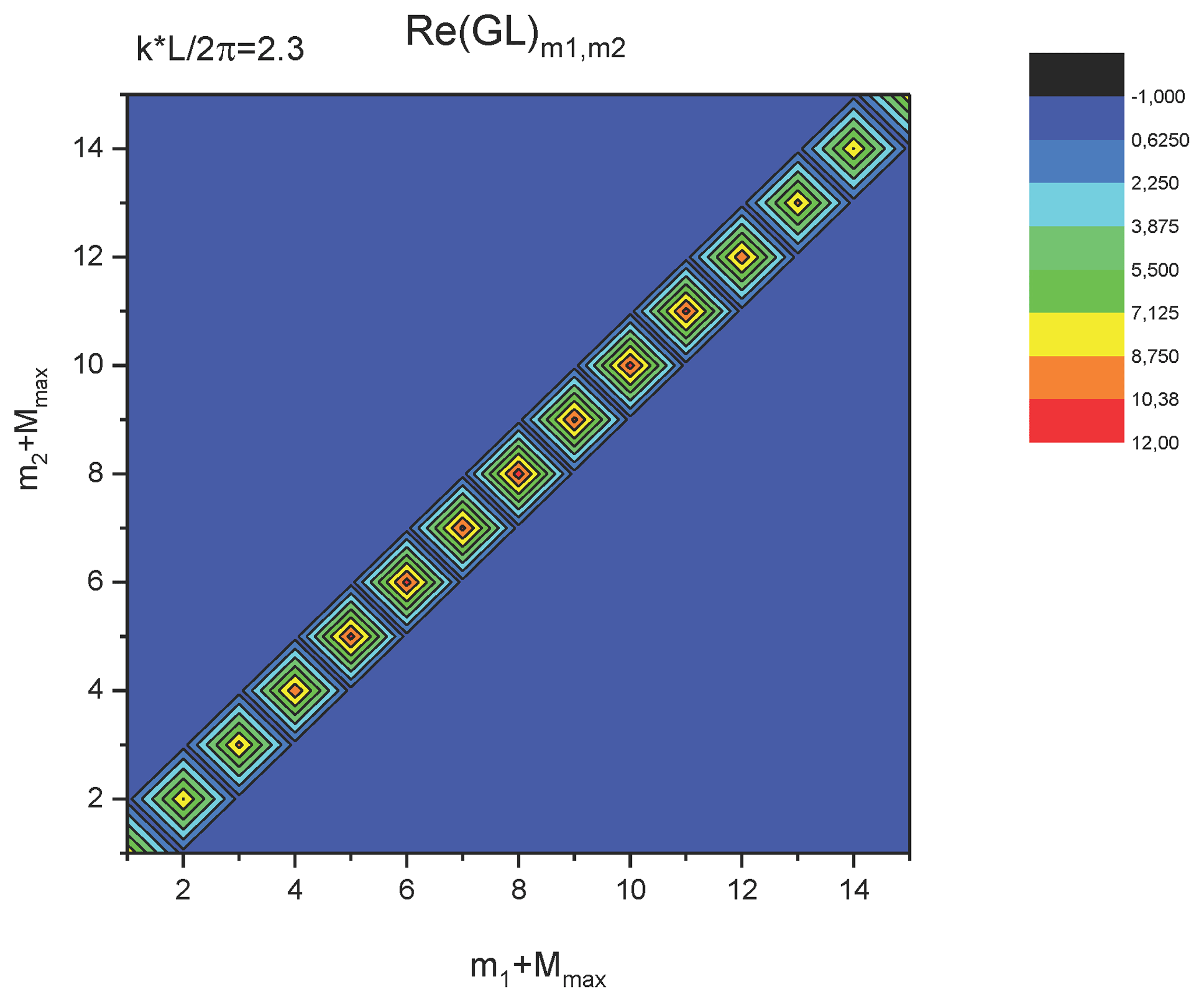
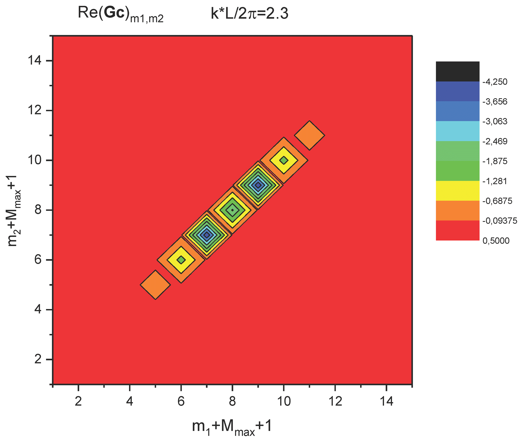
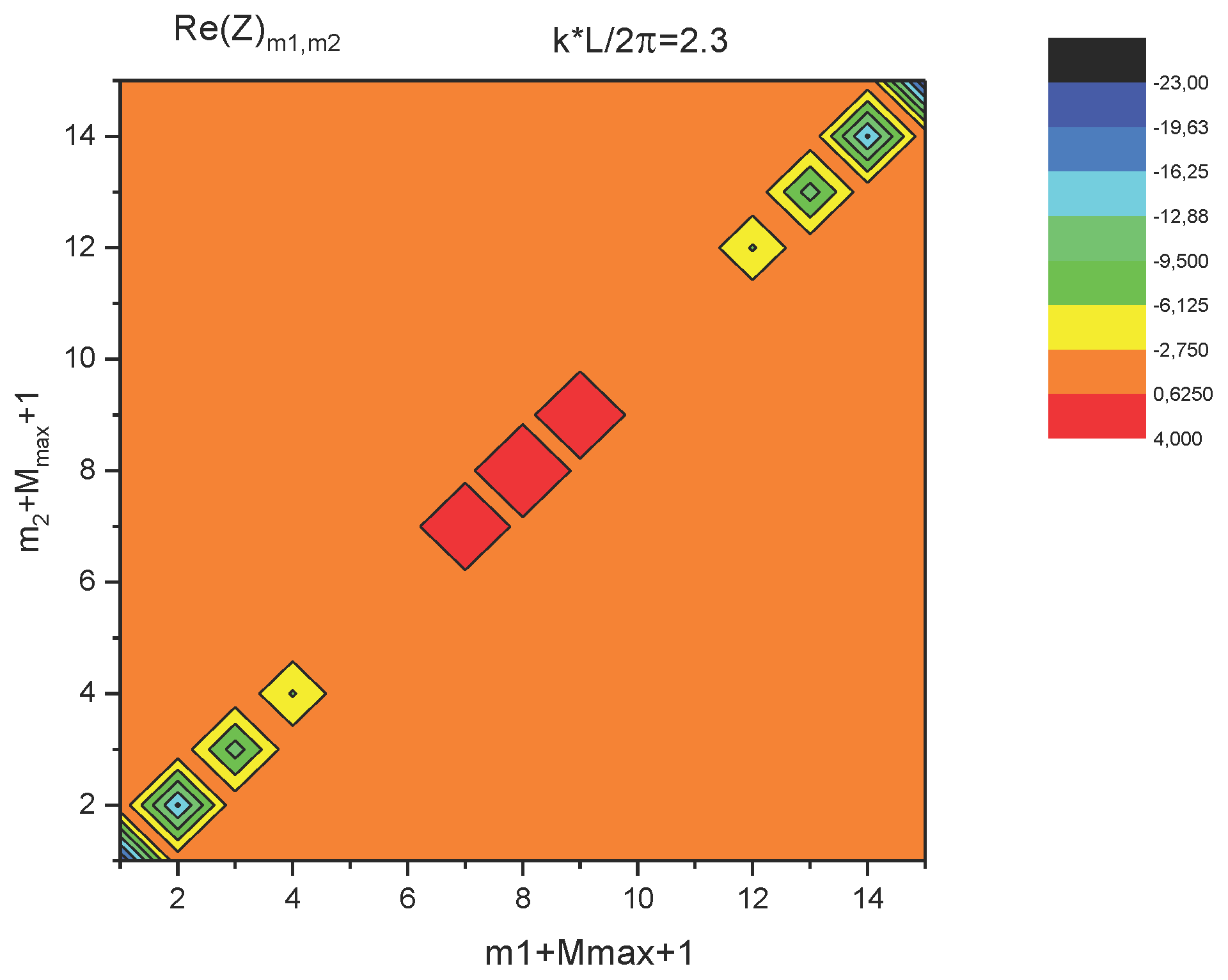
The matrixes G_L and G_C are presented in Fig. 9 for real k. For non-symmetrical configurations, these matrices are not diagonal. However, for the smooth wire ($\mathit{\lambda }\mathrm{|}\mathrm{d}R\left(l\right)/\mathrm{d}l\mathrm{|}\ll \mathrm{|}R\left(l\right)\mathrm{|}$, where R(l) is the radius of curvature of the wire) the number of essential non-diagonal elements is not too big. This can be observed in Fig. 9, especially for the real parts. For the imaginary parts, the non-diagonal elements are essential.

Figure 8 Function $\mathrm{1}/\left|F\right(x,x\left)\right|$ for the elliptical wire.

Figure 9 Matrices G_L (a, b) and G_C (c, d) for semi-elliptical short-circuited wire. $kL/\mathrm{2}\mathit{\pi }=\mathrm{2}/\mathrm{3}$.

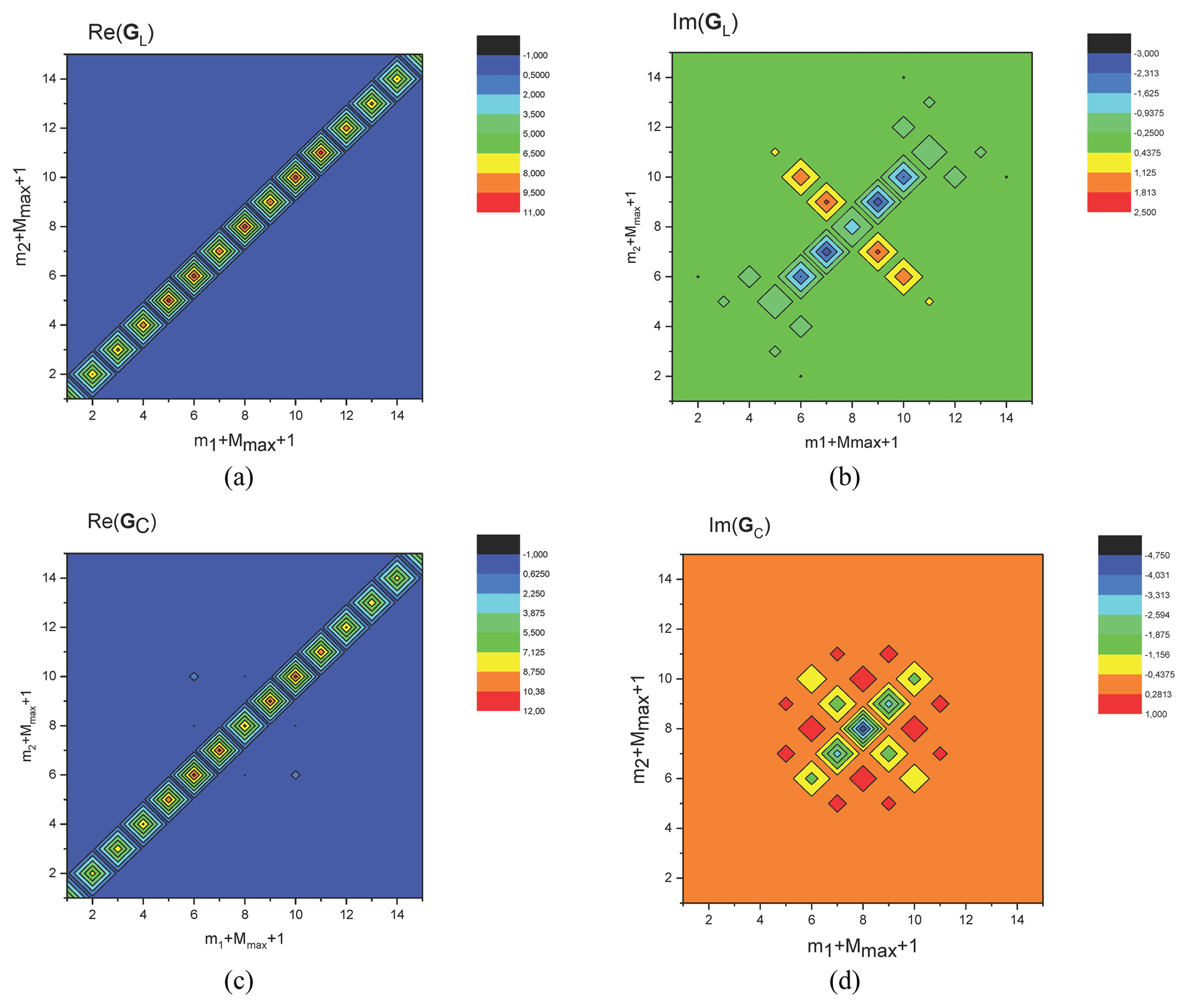
Next, we investigate the symmetry properties of the matrices, which can reduce the time needed to make the calculations. If one looks carefully at the numerical data for the matrix G_C (see Fig. 9c, d), one can see that:

$$\begin{array}{}\text{(20a)}& {\displaystyle }{\left({\mathbf{G}}_C\right)}_{-m\mathrm{1},-m\mathrm{2}}={\left({\mathbf{G}}_C\right)}_{m\mathrm{1},m\mathrm{2}};\text{(20b)}& {\displaystyle }{\left({\mathbf{G}}_C\right)}_{m\mathrm{2},m\mathrm{1}}={\left({\mathbf{G}}_C\right)}_{m\mathrm{1},m\mathrm{2}}\end{array}$$

The same is true for the matrixes G_L(k) and Z(k). This can be proven in the general case. From the definition of G_C(k) we have

$$\begin{array}{}\text{(21)}& \begin{array}{rl}& {\left({\mathbf{G}}_C\right)}_{m\mathrm{1},m\mathrm{2}}=\underset{\mathrm{0}}{\overset{L}{\int }}\underset{\mathrm{0}}{\overset{L}{\int }}{e}^{j{k}_{m\mathrm{1}}{l}_{\mathrm{1}}-j{k}_{m\mathrm{2}}{l}_{\mathrm{2}}}{g}_C(l_{\mathrm{1}},l_{\mathrm{2}},k)\mathrm{d}{l}_{\mathrm{1}}\mathrm{d}{l}_{\mathrm{2}}\\ & \underset{\begin{array}{l}{l}_{\mathrm{1}}->l_{\mathrm{2}}\\ l_{\mathrm{2}}->l_{\mathrm{1}}\end{array}}{=}\underset{\mathrm{0}}{\overset{L}{\int }}\underset{\mathrm{0}}{\overset{L}{\int }}{e}^{j{k}_{m\mathrm{1}}{l}_{\mathrm{2}}-j{k}_{m\mathrm{2}}{l}_{\mathrm{1}}}{g}_C(l_{\mathrm{2}},l_{\mathrm{1}},k)\mathrm{d}{l}_{\mathrm{1}}\mathrm{d}{l}_{\mathrm{2}}\\ & =\underset{\mathrm{0}}{\overset{L}{\int }}\underset{\mathrm{0}}{\overset{L}{\int }}{e}^{j{k}_{m\mathrm{1}}{l}_{\mathrm{2}}-j{k}_{m\mathrm{2}}{l}_{\mathrm{1}}}{g}_C(l_{\mathrm{1}},l_{\mathrm{2}},k)\mathrm{d}{l}_{\mathrm{1}}\mathrm{d}{l}_{\mathrm{2}}\\ & ={\left({\mathbf{G}}_C\right)}_{-m\mathrm{2},-m\mathrm{1}}\end{array}\end{array}$$

Here we used the symmetry property of the scalar Green function when rearranging the arguments $g_C(l_{\mathrm{2}},l_{\mathrm{1}},k)=g_C(l_{\mathrm{1}},l_{\mathrm{2}},k)$.

To prove the property (Eq. 20b) one can write:

$$\begin{array}{}\text{(22)}& \begin{array}{rl}& {\left({\mathbf{G}}_C\right)}_{m\mathrm{1},m\mathrm{2}}:=\underset{\mathrm{0}}{\overset{L}{\int }}\underset{\mathrm{0}}{\overset{L}{\int }}{e}^{j{k}_{m\mathrm{1}}{l}_{\mathrm{1}}-j{k}_{m\mathrm{2}}{l}_{\mathrm{2}}}{g}_C(l_{\mathrm{1}},l_{\mathrm{2}},k)\mathrm{d}{l}_{\mathrm{1}}\mathrm{d}{l}_{\mathrm{2}}\\ & \underset{\begin{array}{l}{l}_{\mathrm{1}}->-l_{\mathrm{1}}\\ l_{\mathrm{2}}->-l_{\mathrm{2}}\end{array}}{=}\underset{\mathrm{0}}{\overset{-L}{\int }}\underset{\mathrm{0}}{\overset{-L}{\int }}{e}^{-j{k}_{m\mathrm{1}}{l}_{\mathrm{1}}+j{k}_{m\mathrm{2}}{l}_{\mathrm{2}}}{g}_C(-l_{\mathrm{1}},-l_{\mathrm{2}},k)\mathrm{d}{l}_{\mathrm{1}}\mathrm{d}{l}_{\mathrm{2}}\\ & =\underset{\mathrm{0}}{\overset{L}{\int }}\underset{\mathrm{0}}{\overset{L}{\int }}{e}^{-j{k}_{m\mathrm{1}}{l}_{\mathrm{1}}+j{k}_{m\mathrm{2}}{l}_{\mathrm{2}}}{g}_C(l_{\mathrm{1}},l_{\mathrm{2}},k)\mathrm{d}{l}_{\mathrm{1}}\mathrm{d}{l}_{\mathrm{2}}\\ & \underset{\begin{array}{l}{l}_{\mathrm{1}}->l_{\mathrm{2}}\\ l_{\mathrm{2}}->l_{\mathrm{1}}\end{array}}{=}\underset{\mathrm{0}}{\overset{L}{\int }}\underset{\mathrm{0}}{\overset{L}{\int }}{e}^{-j{k}_{m\mathrm{1}}{l}_{\mathrm{2}}+j{k}_{m\mathrm{2}}{l}_{\mathrm{1}}}{g}_C(l_{\mathrm{2}},l_{\mathrm{1}},k)\mathrm{d}{l}_{\mathrm{1}}\mathrm{d}{l}_{\mathrm{2}}\\ & =\underset{\mathrm{0}}{\overset{L}{\int }}\underset{\mathrm{0}}{\overset{L}{\int }}{e}^{-j{k}_{m\mathrm{1}}{l}_{\mathrm{2}}+j{k}_{m\mathrm{2}}{l}_{\mathrm{1}}}{g}_C(l_{\mathrm{1}},l_{\mathrm{2}},k)\mathrm{d}{l}_{\mathrm{1}}\mathrm{d}{l}_{\mathrm{2}}\\ & ={\left({\mathbf{G}}_C\right)}_{m\mathrm{2},m\mathrm{1}}\end{array}\end{array}$$

Here we use also the fact of the even number of integrations and the periodic property of all considered functions.

The results of Eqs. (21) and (22) prove the suggestion Eq. (20).

The matrix Z is also non-diagonal. However, near index $m_{\mathrm{eff}}:=kL/\mathrm{2}\mathit{\pi }\approx m(m=\pm \mathrm{1},\pm \mathrm{2},\mathrm{\dots })$ corresponding non-diagonal elements are small. The determinant of this matrix has its minimum for x≈m (see Fig. 8 for the inverse value, which has its maximums). This value serves as a zero-order iteration in the algorithm described above. Using this algorithm, the SEM poles of the first layer were found (Fig. 10). To check the developed method, we compared the results with the SEM poles obtained from the frequency response function of the line obtained using MoM NEC (Numerical Electromagnetic Code) software. The SEM poles can be extracted from numerical data using a Padé approximation, as described by Senior and Pond (1981). The comparison of the poles obtained by the Method of Modal Parameters and proceeding of the data of NEC calculation is shown in Fig. 10.

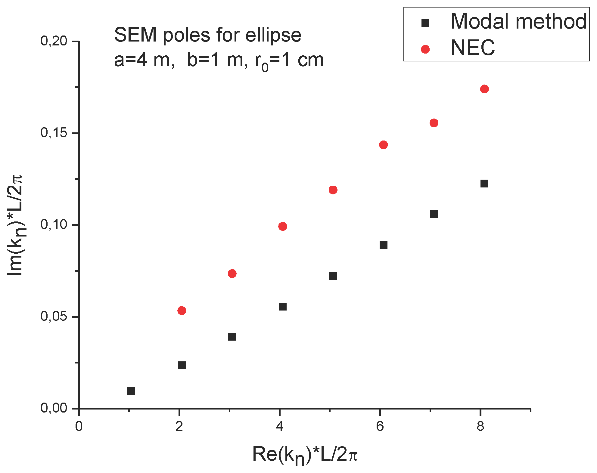
Figure 10 SEM-poles for semielliptical configuration obtained by modal parameter method and by analysis of NEC data.

Figure 11 SEM-poles for semi-circle and semi-elliptical structures. $L_{\mathrm{ellips}}=L_{\mathrm{circle}}=\mathrm{17.1568}$ m.

The comparison of the SEM poles for the semi-elliptical wire with the poles for the semi-circular wire with similar length is shown in Fig. 11. One can see that the imaginary part for the semi-circular wire is essentially larger relative to the semi-elliptical wire. Both sets of poles have a practically linear dependence from the real part. We believe that this is because, in the case of prolate semi-elliptical configuration, the horizontal part of the wire is much closer to the conductive surface, which leads to a weaker radiation, which is ultimately responsible for the appearance of the imaginary part of the SEM poles.

4.3 Straight horizontal wire with short-circuited risers

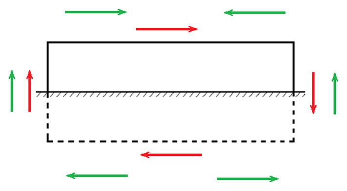
As the third example, we consider another wiring structure, which has many practical applications: the straight horizontal wire with short-circuited risers. We also named this the Vance configuration, because it appears in the book of Edward Vance (1978). The parameters of the line are (Fig. 12): L_hor=10 m, h=0.5 m, r₀=1 cm.

Figure 12 Straight horizontal wire with short-circuited risers.

Figure 13 Function $\mathrm{1}/\left|F\right(x,x\left)\right|$ for the Vance configuration.

The matrixes G_C and G_L for this configuration are presented in Fig. 14. As in the previous example with the prolate elliptic wire, these matrixes contain non-diagonal elements, which, however, are larger than in the previous case, because of the non-smoothness of the line. Nevertheless, the properties of the matrixes (Eqs. 20a, b) are still valid.

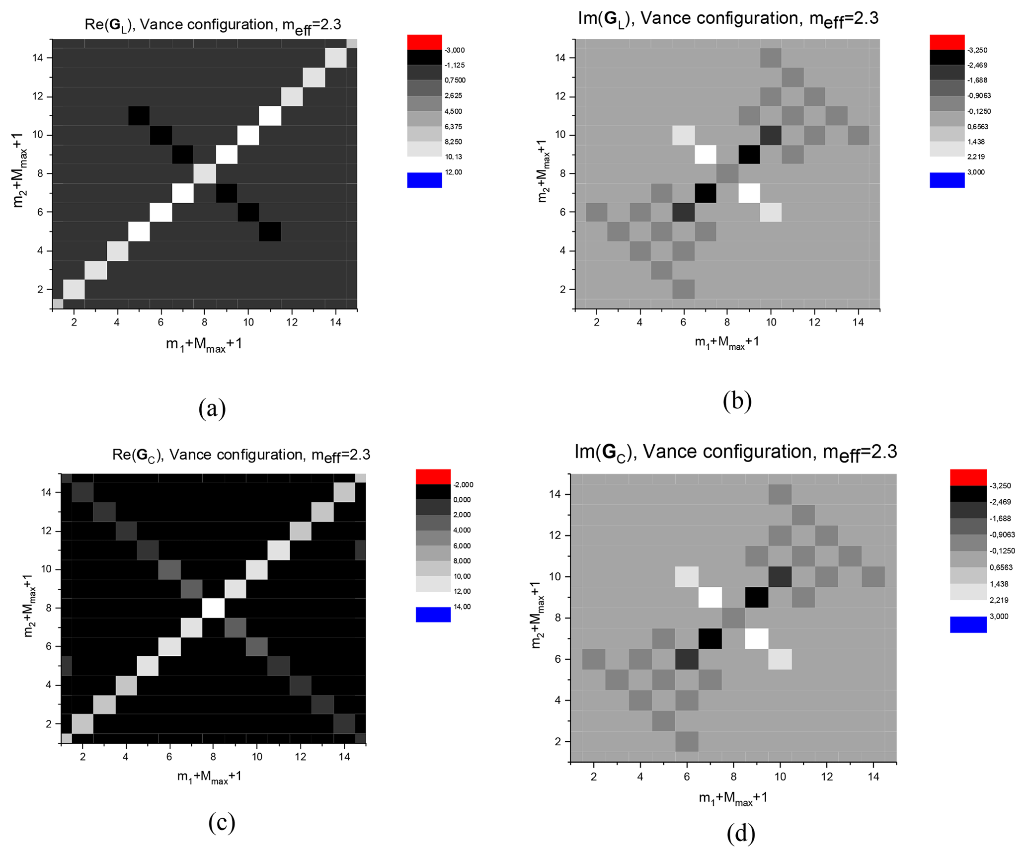
Figure 14 Matrices G_L (a, b) and G_C (c, d) for a straight horizontal wire with short-circuited risers. $kL/\mathrm{2}\mathit{\pi }=\mathrm{2}/\mathrm{3}$.

The frequency dependence of the inverse determinant of the matrix Z (which is also non-diagonal) is shown in Fig. 13. As in the previous cases, it has its maximums near $m_{\mathrm{eff}}:=kL/\mathrm{2}\mathit{\pi }\approx m(m=\pm \mathrm{1},\pm \mathrm{2},\mathrm{\dots })$, which approximately correspond to the real parts of the SEM poles.

Knowledge of the determinant, as a function of complex wave number k, gives us the possibility to determine the SEM poles using the algorithm described above. To check the modal parameter method we compared the results with the one obtained by two alternative methods: the analysis of the response function obtained by NEC (Senior and Pond, 1981), and the asymptotic method (see Tkachenko et al., 2014; Middelstaedt et al., 2016). The results are presented in Fig. 15.

Analyzing the results, we can draw several conclusions. First, the agreement with the “exact” numerical results, as well as with the approximate analytical method is much better in the case of the elliptic wire. This might be caused by the uniform length division by sub-elements in this case, unlike the case of the ellipsoid. In the last case, the uniform division is applied to the parameter t in the usual parametric representation of the ellipse, which leads to a non-uniform division of the lengths of sections of integration and, as a result, the incorrect integration near the singular point at the given number of sub elements (10 000). However, this deficiency can be easily corrected in future calculations.

Figure 15 SEM-poles for the Vance configuration obtained by the modal parameter method, by the asymptotic approach and by analysis of NEC data.

Figure 16 Differential (red color) and common (green color) modes for the Vance structure.

Another important observation is related to the excitation of two types of modes: the common mode and differential mode. The differential mode ($m=\sim \mathrm{0}$, 2, 4, …, see Fig. 15) appears for any transmission line structure, which has horizontal components. The common mode ($m=\sim \mathrm{1}$, 3, 5, …, see Fig. 15) appears for the transmission line structure, which has vertical elements and excited, for example, by an external field, which has vertical components. Note that both types of modes appear in the two previous examples: semi-circular wire and semi-elliptical wire above the perfectly conducting ground with a non-symmetrical excitation. In the case of the wire without vertical components (horizontal open-circuit line above ground), or in the case of a symmetrical configuration (all three considered configurations) and excitation (i.e., plane wave with normal incidence or with grazing incidence), we can observe only one mode type (differential modes or common modes).

The third note is connected with the fact that the presented numerical calculations, using the method of modal parameters is quite a time consuming (for example, the calculation of the 7–10 poles requires 5–6 h on the computer used here). It is possible to show that the modal parameter method allows additional simplification in the case of smooth wires when the radius of curvature of the wire axis is substantially greater than the wavelength. In this case one can introduce for each mode m smoothly length-dependent modal inductance per-unit-length and capacitance per-unit length. These matrices are diagonal (Tkachenko and Nitsch, 2005). The equation for the SEM poles corresponding to the mth mode is given by the diagonal matrix element of the modal impedance per-unit length with the modal functions. It is possible to show that this result can also be obtained by the variation method (Myers et al., 2011a, b). These problems will be addressed in future work.

5 Conclusion

The SEM poles of the short-circuited thin wire with arbitrary geometry above a perfect conducting ground were investigated by the method of modal parameters. Unlike the Method of Moments using the localized basic functions, the method of modal parameters uses physical modal basic functions, which are the approximate solution of MPIE for thin wires, which essentially simplifies finding the poles. The SEM poles are complex roots of the modal impedance matrix of the system. The numerical method of solution of the corresponding equation was developed and applied for several examples: semi-circular wire, semi-elliptical wire, and horizontal wire with vertical risers. During this procedure, matrices of modal inductance and capacitance were calculated and their symmetry was investigated. The comparison of the SEM poles with the ones obtained by other analytical and numerical methods yields a good agreement. The causes of the disagreement with the numerical results are analyzed. The main cause is using matrices that are not sufficiently large. In our opinion, it possible to improve results by accelerating calculations using the symmetry properties of modal matrixes (Eqs. 20a, b).

Note, that the MoMP can also be applied for the open-circuited wire if one uses a different modal function (sine and cosine). In the future, the developed method can be generalized for the case of a loaded wire by including the lumped impedances as current controlled voltage sources.