Near-field measurement of continuously modulated fields employing the time-harmonic near- to far-field transformation

Near-field far-field transformations (NFFFTs) are commonly performed for time-harmonic fields. Considering arbitrary in-situ measurement scenarios with given transmission signals, time-varying aspects of modulated signals have to be taken into consideration. We investigate and characterize two methods for the measurement of modulated fields, which work with a time-domain representation of the radiated fields and, at the same time, allow to employ the standard time-harmonic NFFFT. One method is based on the fact that the modulation signal can be assumed to be constant in a short enough measurement interval under the condition that the modulation and carrier frequencies are several decades apart. The second method performs long-time measurements in order to obtain the complete frequency spectrum in every single measurement. Both methods are verified by the NFFFT of synthetic field data.

1 Introduction

With the rise of wireless communication technologies, also the demand for antenna characterization increases. One of the most important characteristics of an antenna is its far-field (FF) radiation pattern. A common method to obtain the radiation pattern involves near-field (NF) measurements of the antenna from which the FF can be calculated in the post-processing. This is known as the NF to FF transformation (NFFFT) (Yaghjian, 1986), where advanced algorithms such as the fast irregular antenna field transformation algorithm (FIAFTA) offer various source representations and additional diagnostic capabilities (Schmidt et al., 2008; Eibert et al., 2015). NF measurements are usually performed in anechoic chambers, since they provide an echo free measurement environment, which forms a defined and acceptable approximation of free space. However, it is sometimes necessary to perform in-situ measurements, especially if an antenna is too large to be mounted in available anechoic chambers or if an antenna shall be measured in its real environment. In such more natural environments, the FIAFTA offers modelling capabilities suitable for in-situ measurements, like handling a reflective ground (Mauermayer and Eibert, 2018; Eibert and Mauermayer, 2018) as well as echo suppression of known and unknown scatterers (Yinusa and Eibert, 2013). In-situ measurements can be, for example, perfomed with unmanned aerial vehicles (UAVs), where a large problem is that common receiver equipment can easily measure only the magnitudes of the fields (Virone et al., 2014; Fritzel et al., 2016; García-Fernández et al., 2017). Since available algorithms for phaseless NFFFT are not yet completely reliable (Paulus et al., 2017), we assume an in-situ measurement scenario where magnitude and phase are available.

In this work, we tackle the problem of handling modulated fields arising in in-situ measurements. To do so, NFFFT algorithms are reviewed first. For time-harmonic fields, the NFFFT can be formulated as a linear inverse problem, where equivalent sources, e.g., equivalent surface current densities on a surface enclosing the AUT, plane wave spectra or spherical multipoles, are to be retrieved. Solving this inverse problem, an equivalent source model is attained that reconstructs the measured NF and from which the FF is calculated. State-of-the-art algorithms for time-harmonic signals work in the spectral domain, i.e., for single-frequency signals. For modulated signals, the single-frequency assumption does not hold any more. Even if there are NFFFT algorithms that work in the time domain and can deal with modulated fields (Oetting and Klinkenbusch, 2005), most NFFFTs deal with time-harmonic fields and work in the frequency domain. Further, frequency domain NFFFTs are usually faster and more efficient than their time-domain counterparts. To overcome this problem, we present two methods to measure or process the time-varying electromagnetic fields in a way that they can be used in a time-harmonic NFFFT algorithm. Still, the application we have in mind are UAV-based in-situ measurements of modulated signals. Worth mentioning is a certain drawback of UAVs which are normally not able to hover at a specific position for a longer time. This leads to errors due to some uncertainty in the position of the NF measurements which depends on the measurement time. Therefore, the measurement time must be kept as short as possible in UAV-based measurement setups.

The paper is structured as follows. In Sect. 2, the Fourier transform and the specialties of the measurement of time-varying fields are briefly reviewed. Then, two different techniques to measure modulated fields are described and compared. In both cases, the NFFFT is based on the common time-harmonic NFFFT, in particular the FIAFTA. Finally, in Sect. 3, transformation results of synthetic NF data show the validity of both measurement techniques.

2 Transformation of continuously modulated fields by employing the time-harmonic NFFFT

To cope with continuously modulated (i.e. continuously time-varying with a certain periodicity and without abrupt phase and magnitude changes) fields within the time-harmonic NFFFT, the field signals must be available in the frequency domain. In this work, we concentrate on the case of continuously amplitude modulated fields. This is only for the reason of simplicity and demonstration as all investigations hold true for the generic case. A continuously modulated field

$$\begin{array}{}\text{(1)}& E(t,{\mathit{r}}_{\mathrm{0}})=m\left(t\right)E\left({\mathit{r}}_{\mathrm{0}}\right)\cos \left(\mathrm{2}\mathit{\pi }{f}_{\mathrm{c}}t+{\mathit{\varphi }}_{\mathrm{0}}\right)\end{array}$$

dependent on time t and a specific position r₀, is considered. m(t) is the time-varying modulation signal, E(r₀) the field amplitude evaluated at the position r₀ but constant in time, f_c is the carrier frequency of the field signal and ϕ₀ is the carrier phase. In general, the relation between time and frequency domain is given by the Fourier transform, which is

$$\begin{array}{}\text{(2)}& X\left(f\right)=\underset{-\mathrm{\infty }}{\overset{\mathrm{\infty }}{\int }}x\left(t\right){\mathrm{e}}^{-\mathrm{j}\mathrm{2}\mathit{\pi }ft}\mathrm{d}t\end{array}$$

and, its inverse

$$\begin{array}{}\text{(3)}& x\left(t\right)=\underset{-\mathrm{\infty }}{\overset{\mathrm{\infty }}{\int }}X\left(f\right){\mathrm{e}}^{\mathrm{j}\mathrm{2}\mathit{\pi }ft}\mathrm{d}f,\end{array}$$

where f is the frequency, x(t) the time-domain signal and X(f) its corresponding frequency spectrum. However, when it comes to the measurement of real-world signals, a window function w(t) should be introduced which is only non-zero in the measurement interval and vanishes outside. w(t) is considered as a rectangular window for the transformation of finite-length signals. Regarding the window function, Eq. (2) changes to

$$\begin{array}{}\text{(4)}& X(\mathit{\tau },f)=\underset{-\mathrm{\infty }}{\overset{\mathrm{\infty }}{\int }}x\left(t\right)w(t-\mathit{\tau }){\mathrm{e}}^{-\mathrm{j}\mathrm{2}\mathit{\pi }ft}\mathrm{d}t,\end{array}$$

which is known as the short-time Fourier transform (STFT) (Allen, 1977). The opening time of w(t) is directly related to the measurement time, which is relevant for the following subsections.

2.1 Long-time measurement approach

One approach towards the NFFFT of modulated fields is to measure the field signal in the time-domain for such a long time that all relevant frequency components can be resolved and distinguished, followed by a Fourier transform. This approach is called long-time measurement (LTM) in the following. Within the LTM, the Fourier transform is performed for every measurement position which results in a frequency spectrum per position. From all spectra together, one frequency component can be extracted and transformed to the FF by virtue of the time-harmonic NFFFT. This is repeated for all frequencies present in the field signal. In the FF, the spectrum can be composed of the different frequency components which have been transformed by the NFFFT. An inverse Fourier transform eventually results in the time-varying FF. The principle consists of four steps and is illustrated in Fig. 1.

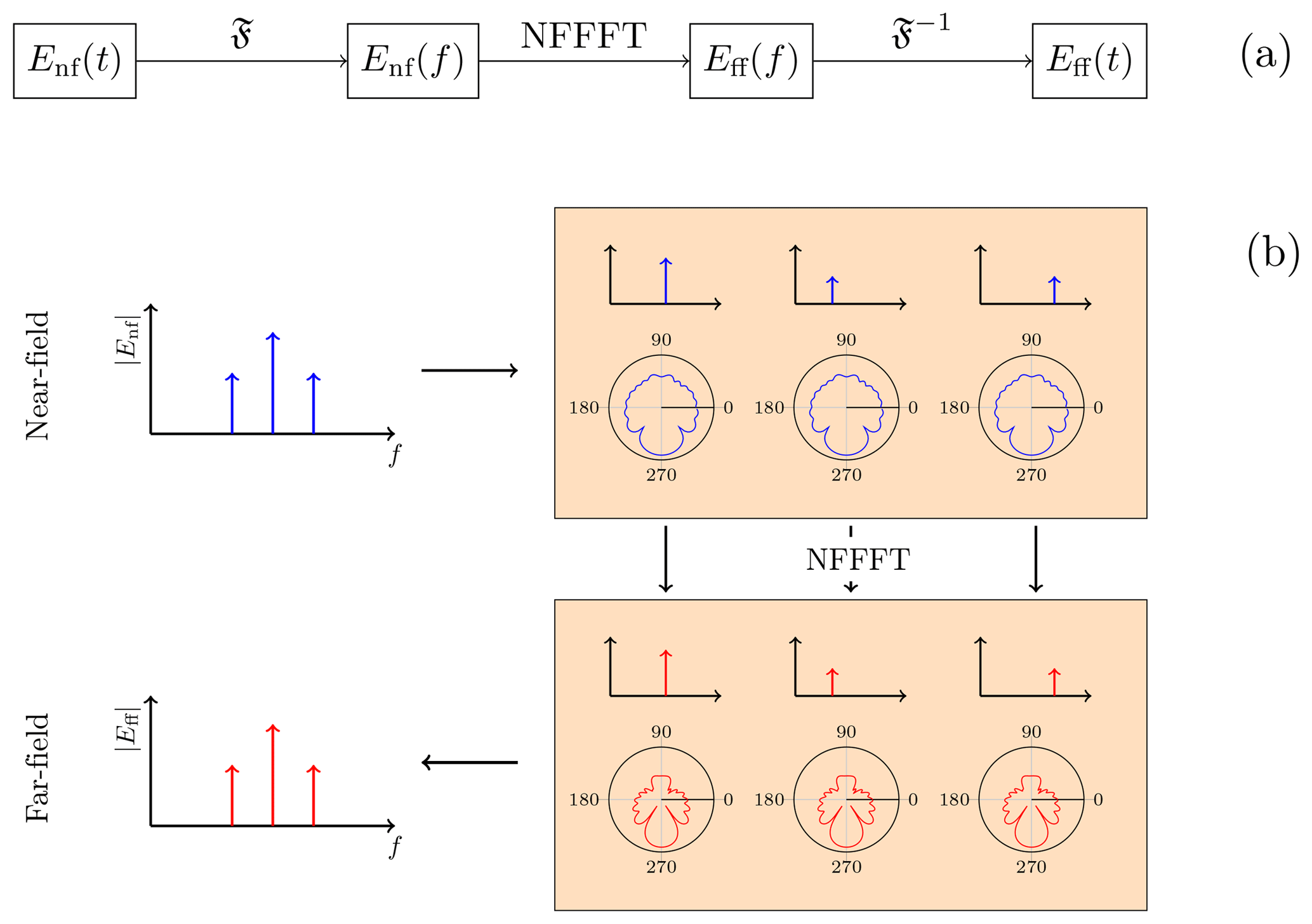
Figure 1 The long-time measurement approach consists of four steps (a) where the field signal is present in different forms. The NF signal is measured in the time-domain and the frequency spectrum is calculated by the Fourier transform for every measurement position. Then, the single frequency components are extracted and transformed to the far-field by using the NFFFT (b). Each frequency component consists of a full transformable set of NF samples. The single-frequency FFs, which result from the NFFFTs, are composed together in the FF frequency spectrum. Eventually, an inverse Fourier transform gives the time-domain FF.

The LTM technique relies in particular on the fact that the amplitude and phase relations between the single frequency components are retained throughout the complete processing chain, from the measurement, no matter whether in time domain or in frequency domain, over the NFFFT, until the final signal composition in the FF.

A drawback of the method is the measurement time T_meas, i.e., the width of the window function w(t) in Eq. (4), which is required to record the field at one position. T_meas, in turn, defines the achievable frequency resolution Δf, i.e., the difference in frequency that is distinguishable in the spectral domain. The relation between T_meas and Δf is a consequence of Küpfmüller's uncertainty principle (Hoffmann, 2005) and is

$$\begin{array}{}\text{(5)}& T_{\mathrm{meas}}\ge {\displaystyle \frac{\mathrm{1}}{\mathrm{\Delta }f}}.\end{array}$$

This implies that T_meas can become very long when a fine frequency resolution is necessary to correctly model the spectral behavior of the measured signal.

2.2 Short-time measurement approach

In contrast to the LTM, the width of the window function can also be chosen much shorter. This basically avoids the issue of long measurement times but brings along other effects which have to be treated carefully. If T_meas is chosen to be shorter than required by Eq. (5), the single frequency components are indistinguishable in the spectrum. However, if T_meas is further reduced to such a short time span that the modulation present in the field signal can be considered to be constant in the measurement interval, effectively only the carrier signal is measured. This is illustrated in Fig. 2.

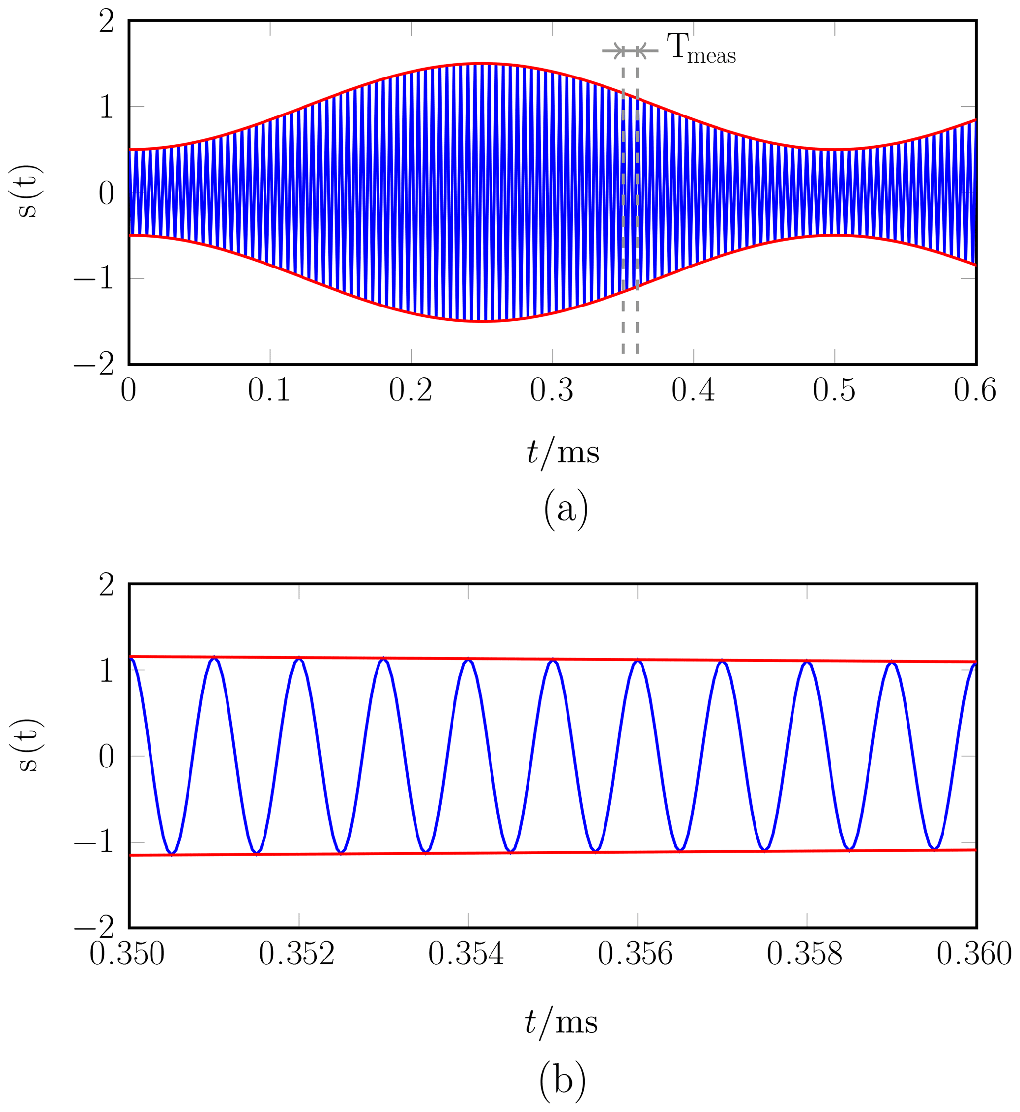
Figure 2 Within the short-time measurement approach, the field signal (a) is measured for such a short time that the modulation signal can be treated as constant during the measurement interval (b). Here, an amplitude modulated signal with modulation frequency 2 Hz and carrier frequency 1 kHz is shown. (The carrier frequency in (a) has been scaled for better readability.)

Assuming a constant modulation signal m_i=m(t_i) during the ith measurement interval around a certain time stamp t_i, Eq. (1) changes to

$$\begin{array}{}\text{(6)}& E(t,{\mathit{r}}_{\mathrm{0}})=m_{i}E\left({\mathit{r}}_{\mathrm{0}}\right)\cos \left(\mathrm{2}\mathit{\pi }{f}_{\mathrm{c}}t+{\mathit{\varphi }}_{\mathrm{0}}\right).\end{array}$$

This means that the envelope of the modulated field signal is sampled by every measurement. The result is a time-harmonic field value at the carrier frequency of the field signal, weighted with the constant factor m_i. If the whole time-varying NF is sampled in this way, all measurement samples that share the same constant weighting factor m_i build a set of field values with the same modulation state. This is for instance possible if the modulation signal m(t) is periodic with T_m, i.e.,

$$\begin{array}{}\text{(7)}& m\left(t_i\right)=m(t_i+T_{\mathrm{m}}).\end{array}$$

The modulation signal could be for example an amplitude modulation

$$\begin{array}{}\text{(8)}& m\left(t\right)=A\cos \left(\mathrm{2}\mathit{\pi }{f}_{\mathrm{m}}t+{\mathit{\varphi }}_{\mathrm{m}}\right),\end{array}$$

where A is a constant amplitude factor, f_m the modulation frequency and ϕ_m the phase of the modulation signal. The measured NF data sets can be used for the field transformation with the time-harmonic NFFFT algorithm. Due to the linearity of the field transformation, the far-field will also be weighted by the same constant factor m_i. The consecutive measurement and transformation of different modulation states results in the time varying far-field signal, see Fig. 3.

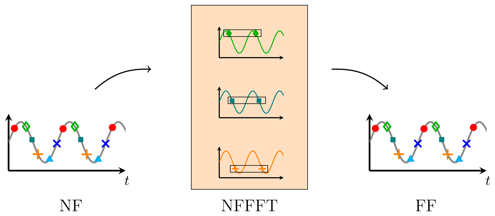
Figure 3 Principle of the short-time measurement approach. The envelope of the time-varying field signal is sampled by each measurement. All samples sharing the same modulation state are transformed as a data set to the FF, which is equivalent to the transformation of the single frequency components within the LTM in Fig. 1b. Measurements and transformations of consecutive modulation states leads to the time-varying FF.

Since this technique requires a shorter measurement time and allows for a faster measurement, it is called short-time measurement (STM) in the following. The advantage of the STM over the LTM approach is the shorter measurement time which makes this approach suitable for field measurements with UAVs. Due to the short measurement time, we assume that position changes of an employed UAV play no role and that the modulation signal does not change significantly during the measurement interval. The short measurement time implies a broader bandwidth (according to Eq. 5) than for the LTM. In particular, the measurement bandwidth has to be larger than the signal/modulation bandwidth. A necessary condition is that the carrier frequency f_c is much higher than the modulation frequency f_m. If this condition holds, the measurement interval still contains several periods of the carrier signal, but the modulation signal is assumed to be constant during the measurement interval. Such a scenario is depicted in Fig. 2.

Further, both approaches work only if the time-varying field signal is periodic since one transformable field data set consists of components from multiple measurements which have to be taken one after the other. Even if the measurement time can be short for single measurements, the reconstruction of the modulation signal requires that the sampling theorem is fulfilled for consecutive measurements. This is due to the fact that the STM is a sampling of the signal envelope. Therefore, the sampling theorem is given by (Gibson, 1993)

$$\begin{array}{}\text{(9)}& \mathrm{\Delta }T>{\displaystyle \frac{\mathrm{1}}{\mathrm{2}{f}_{\mathrm{m}}}}\end{array}$$

where ΔT is the time between two consecutive measurements.

Sometimes it may be assumed that the far-field radiation pattern for the carrier frequency and for the modulation sidebands does not change significantly, since f_c≫f_m. In this case and when only the far-field radiation pattern at f_c is of interest, the STM approach can be simplified. The field at the carrier frequency can be determined by dividing the measured field value by the modulation factor m(t_meas) resulting in

$$\begin{array}{}\text{(10)}& E\left(t_{\mathrm{meas}},{\mathit{r}}_{\mathrm{0}}\right)={\displaystyle \frac{m\left(t_{\mathrm{meas}}\right)E\left({\mathit{r}}_{\mathrm{0}}\right)\cos \left(\mathrm{2}\mathit{\pi }{f}_{\mathrm{c}}t+{\mathit{\varphi }}_{\mathrm{0}}\right)}{m\left(t_{\mathrm{meas}}\right)}}.\end{array}$$

3 Simulation results

The applicability of the STM and LTM approaches is demonstrated by numerical results. The NF data is generated synthetically from a horn antenna that is represented by Hertzian dipoles. To create a realistic antenna model, the surface currents of a time-harmonic full-wave simulation of the horn antenna were approximated by 2232 Hertzian dipoles on the PEC surface. The full-wave simulation was performed in CST Microwave Studio (CST, 2014) at a frequency of 3 GHz. Figure 4 shows the arrangement and locations of the dipoles.

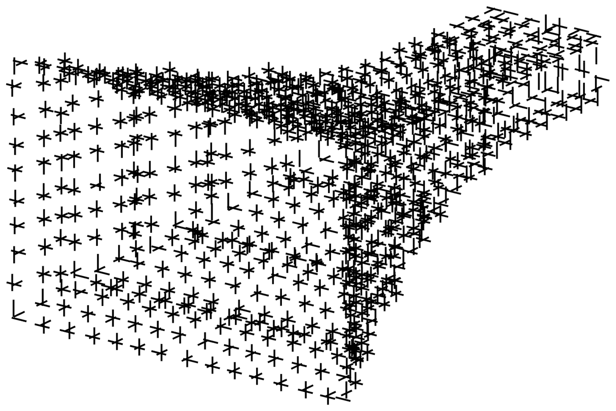
Figure 4 Arrangement of the 2232 Hertzian dipoles that represent a horn antenna. The excitation of the Hertzian dipoles has been found from the discretization of the horn antenna's surface currents.

The antenna has an aperture of 222.4 mm × 148.27 mm and is operated in transmit mode with an amplitude modulated (AM) signal s(t) at a carrier frequency of f_c=3 GHz. The AM-signal is given by

$$\begin{array}{}\text{(11)}& s\left(t\right)=\left(\mathrm{1}+M\cos \left(\mathrm{2}\mathit{\pi }{f}_{\mathrm{m}}t+{\mathit{\varphi }}_{\mathrm{m}}\right)\right)\cos \left(\mathrm{2}\mathit{\pi }{f}_{\mathrm{c}}t+{\mathit{\varphi }}_{\mathrm{0}}\right),\end{array}$$

where M=0.5 is the modulation index and f_m=200 Hz the modulation frequency. The modulation phase has been chosen to ϕ_m=0 for the presented simulations but other phases have also been tested. Since the model uses time-harmonic Hertzian dipoles, the AM is introduced by calculating the fields from the dipole model for the carrier frequency f_c as well as for the upper and lower sideband frequencies f_c±f_m, where all dipoles are modulated synchronously. The time-varying NFs are then computed by the inverse Fourier transform Eq. (3) regarding their frequencies. Here, the excitation of the Hertzian dipoles was chosen according to the currents found from the full-wave simulation as described before. Starting with the time signal, the synthetic time-varying NF is processed according to the STM and LTM approaches and a NFFFT is performed using FIAFTA.

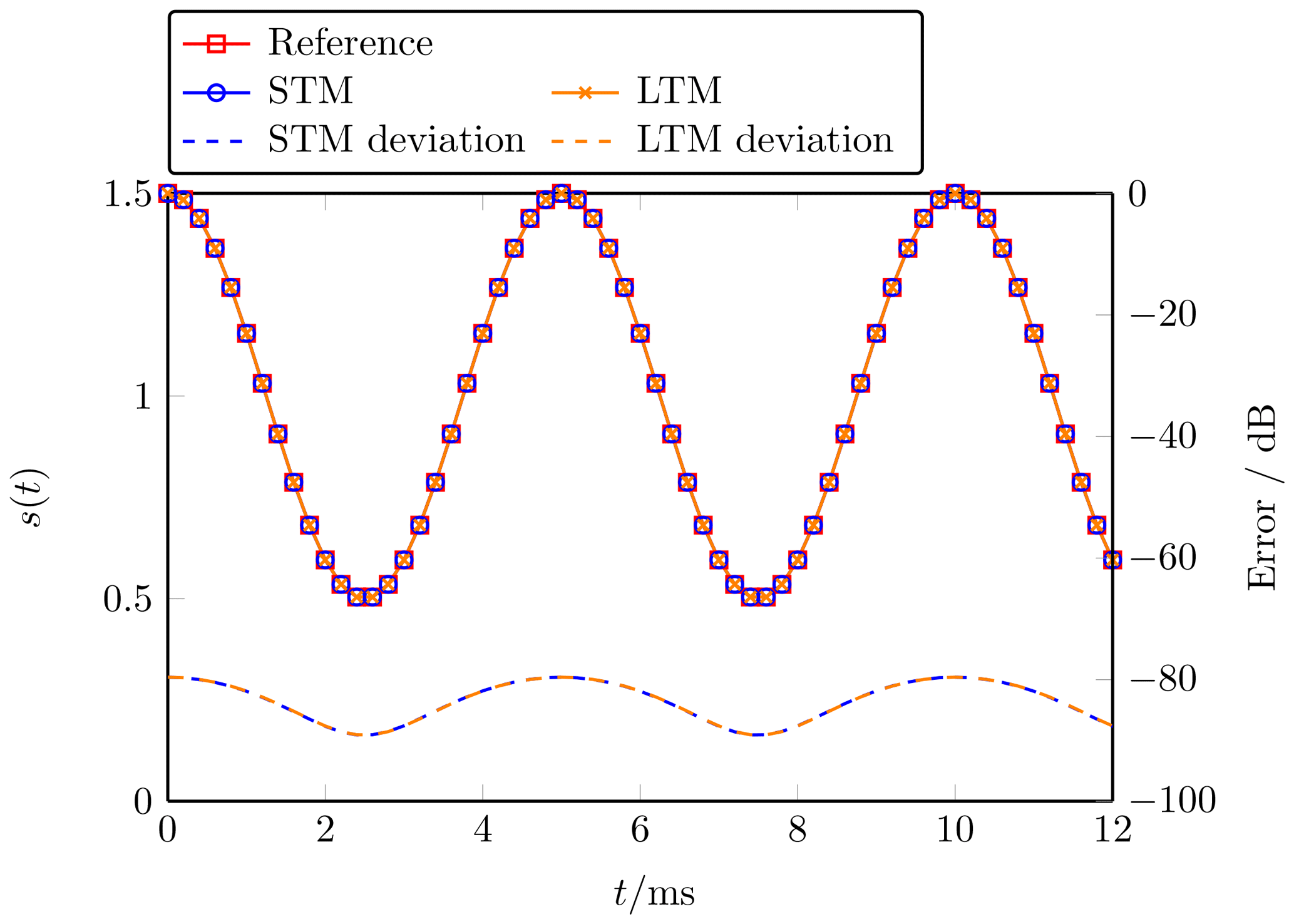
Figure 5 Time-varying far-field signal at the center of the AUT main beam. The transformed fields of the STM (blue) and LTM (orange) match with the reference (red) signal. Both approaches do not introduce any additional error to the field measurement, the resulting error is due to the NFFFT.

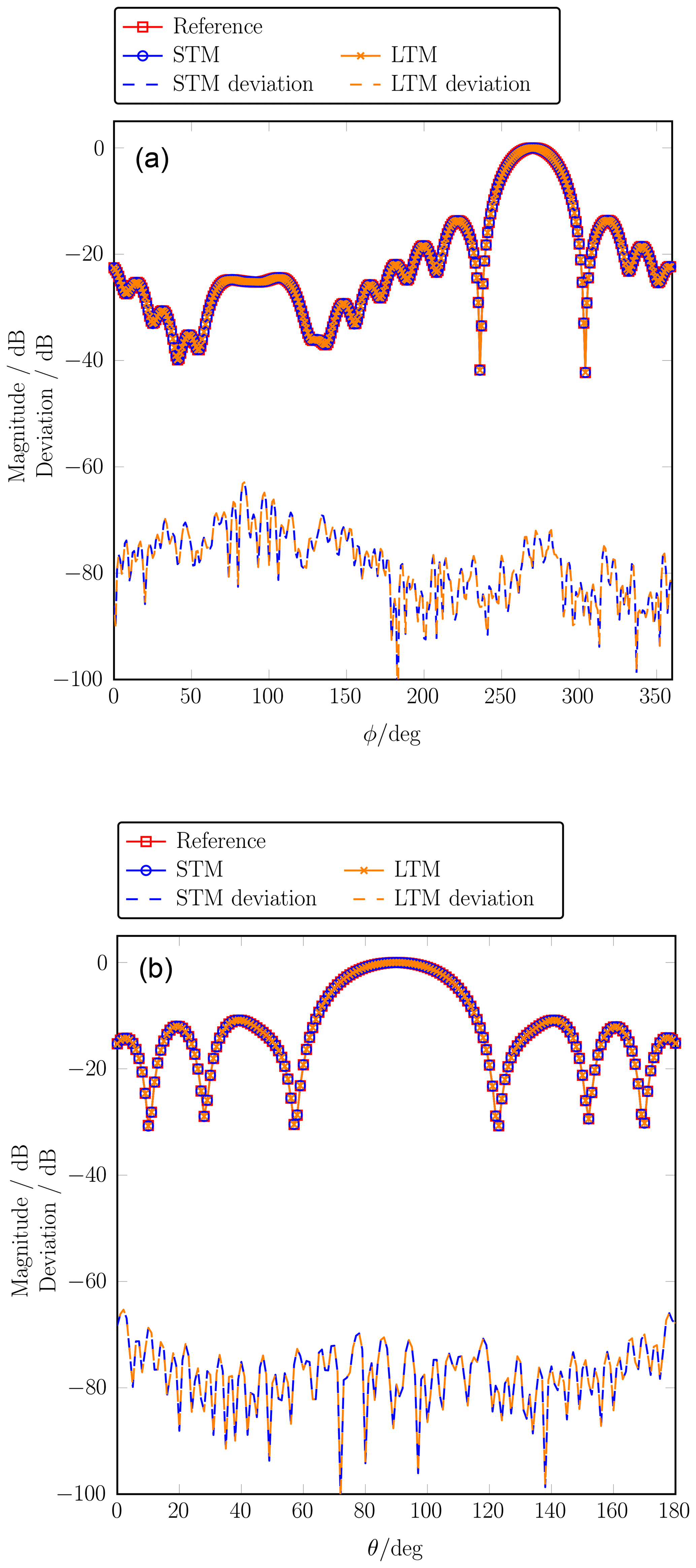
Figure 6 Far-field main cuts at the carrier frequency in comparison with a reference pattern obtained from a time-harmonic simulation. The phi-cut (a) is evaluated at $\mathit{\theta }=\mathrm{90}{}^{\circ }$ and the theta-cut (b) at $\mathit{\varphi }=\mathrm{270}{}^{\circ }$. The maximum deviation of the STM and LTM approach from the reference is −62 dB, which is equal to the error of the NFFFT.

Figure 5 shows the FF time signal at the center point $(\mathit{\theta }=\mathrm{90}{}^{\circ },\mathit{\varphi }=\mathrm{270}{}^{\circ })$ of the main beam of the horn antenna for the co-polarization E_θ. The reference signal has been calculated directly from the dipole model, using the FF approximation for Hertzian dipoles, see Balanis (2005). The STM time signal is attained via a series of NFFFTs as described in Sect. 2.2. Each marker corresponds to one NFFFT and 100 calculations have been performed in total. The LTM time signal is calculated as the inverse Fourier transform from the FF frequency spectrum as described in Sect. 2.1. The deviation of the STM and LTM from the reference signal is calculated by

$$\begin{array}{}\text{(12)}& \mathit{ϵ}=\mathrm{20}\log \left(\right|{\displaystyle \frac{E_{\mathrm{ref}}}{max\left(\left|E_{\mathrm{ref}}\right|\right)}}-{\displaystyle \frac{E_{\mathrm{STM}/\mathrm{LTM}}}{max\left(\left|E_{\mathrm{STM}/\mathrm{LTM}}\right|\right)}}\left|\right),\end{array}$$

where E_ref is the reference FF signal obtained directly from the dipole model and E_STM∕LTM is the FF signal obtained from the STM and LTM. The highest errors for the STM and the LTM are below −80 dB in this plot. However, considering all radiation directions the largest error between the STM ∕ LTM and the reference signal is −62 dB. This error is equal to the error of the NFFFT, which means that both, STM and LTM, do not introduce any noticeable error to the data. This is expected since the sampling theorem is fulfilled.

The FF main cuts at the carrier frequency are depicted in Fig. 6. The carrier frequency FF of the STM is calculated according to Eq. (10) while the carrier frequency can be extracted directly from the frequency spectrum within the LTM. The error of both measurement techniques is also shown.

A key difference between the STM and the LTM is the actual measurement time. Lacking a real-world measurement scenario, this can be only estimated based on the presented example. For the LTM, the field signal has been measured at each position for a time span of ΔT_LTM=40 ms which includes several modulation periods. Since there are N=11250 measurement locations, the total measurement time for the LTM is estimated to $T_{\mathrm{LTM}}=N\mathrm{\Delta }{T}_{\mathrm{LTM}}=\mathrm{450}\mathrm{s}$. In the simulation for the STM, the time interval of a single measurement is considered to be ideally zero, which does not change the measurement principle but reduces computation time. However, a realistic measurement time for the STM in the simulated example is ΔT_STM=100 µs, which corresponds to a measurement bandwidth of 10 kHz. Further, in the example 100 times more field samples have been used for the STM in comparison to the LTM to ensure collecting all modulation states at all positions. In sum, this results in an overall measurement time of $T_{\mathrm{STM}}=\mathrm{100}N\mathrm{\Delta }{T}_{\mathrm{STM}}=\mathrm{112.5}\mathrm{s}$ for the STM. However, certainly, the positioning will take most of the time in this example but the STM seems to be in advantage regarding pure measurement time.

4 Conclusions

Two different techniques for the measurement of modulated fields have been presented, which both extend the time-harmonic NFFFT to the case of modulated electromagnetic fields. The validity of the measurement approaches was shown by NFFFTs of synthetically generated NF data of a horn antenna model. It has been demonstrated that the resulting deviation of the LTM and STM are on a very similar accuracy level and that the introduced error does not significantly deviate from the error of the single-frequency-time-harmonic NFFFT. Comparing the two methods, the advantage of the STM over the LTM is the faster measurement time, which enables the use of this technique for UAV-based antenna measurements and other applications where short measurement times are mandatory.