Characteristic Mode Analysis of surface current distributions on metallic structures exposed to HIRF- and DCI-excitations

This paper treats Characteristic Mode Analyses of three-dimensional test objects in the context of EMC. Based on computed Characteristic Modes and mode-specific physical quantities, series expansions for HIRF- and DCI-induced surface currents are deduced. The contribution of single Characteristic Modes to surface currents at different test frequencies is analyzed. HIRF- and DCI-excitations are compared with regard to their surface current distributions in their resonance region determined by Characteristic Mode Analysis.

1 Introduction

Radiated immunity tests in anechoic chambers using HIRF (High Intensity Radiated Field) are a common EMC test procedure in the automotive sector described in DIN EN 61000-4-3 (2011). Related test environments include TEM waveguides specified by DIN EN 61000-4-20 (2010) and reverberation chambers, see DIN EN 61000-4-21 (2011), all of which are based on radiation coupling to a device under test (DUT).

In the recent past, a conducted alternative called DCI (Direct Current Injection), also refered to as Direct Drive in ED-107A (2015) found application in immunity testing. With the help of adapters galvanically coupled to a DUT, currents are directly injected onto its surface, see Leat (2007) for an exemplary test scenario. In this manner, DCI seeks to approximate the surface currents on DUTs generated during HIRF tests. As mathematical background serves the surface equivalence principle proving that identical charge or current distributions on an object's surface cause equal fields within its interior volume, see Harrington (2001). In general, EMC testing is most critical when a DUT is excited at its resonance frequencies. Characteristic Mode Analysis (CMA) is a tool that allows to determine the resonances of a system, characterized by so called Characteristic Modes. Since both HIRF and DCI test setups differ from each other geometrically, both sets of Characteristic Modes cannot coincide with each other, thus making DCI only an approximation to HIRF.

Other than most publications in which CMA has been applied to antenna design, see e.g. Vogel et al. (2015), EMC testing is addressed in this paper. Herefore, explicit mathematical expressions for surface currents of HIRF and DCI setups expanded in Characteristic Modes are deduced. In doing so, it is quantitatively investigated in how far Characteristic Modes determine surface current distributions in EMC tests at resonance and beyond.

The following sections are introduced by a summary on the theoretical background of CMA. It is subsequently applied on various test objects in HIRF- and DCI-configuration, starting off with a cylinder as generic test object. Finally, as more realistic test object, a car geometry is investigated.

2 Characteristic Mode Analysis

The mathematical foundations of Characteristic Mode Analysis are covered in Harrington and Mautz (1971). The basic problem to solve in CMA is the generalized eigenvalue problem

$$\begin{array}{}\text{(1)}& \mathbf{X}{\mathit{J}}_n={\mathit{\lambda }}_n\mathbf{R}{\mathit{J}}_n\end{array}$$

with ${\mathit{J}}_n,n\in \mathbb{N}$ signifying real-valued eigenfunctions called Characteristic Modes to determine, as are the eigenvalues ${\mathit{\lambda }}_n\in [-\mathrm{\infty },\mathrm{\infty }]$. Matrices R and X are real and imaginary parts of the system's impedance matrix $\underset{\mathrm{¯}}{\mathbf{Z}}=\mathbf{R}+\mathrm{j}\mathbf{X}$.All Characteristic Modes J_n are orthonormal to one another with reference to the resistance matrix R,

$$\begin{array}{}\text{(2)}& 〈{\mathit{J}}_m,\mathbf{R}{\mathit{J}}_n〉={\mathit{\delta }}_{mn}=\left\{\begin{array}{ll}\mathrm{1}& \text{for}m=n\\ \mathrm{0}& \text{for}m\ne n\end{array}\right.,\end{array}$$

and can thus serve as basis for a Fourier series expansion of the total surface current $\underset{\mathrm{¯}}{\mathit{J}}\left(\mathit{r}\right)$ generated in HIRF and DCI tests according to

$$\begin{array}{}\text{(3)}& \underset{\mathrm{¯}}{\mathit{J}}\left(\mathit{r}\right)=\sum _{n=\mathrm{1}}^{\mathrm{\infty }}{\underset{\mathrm{¯}}{\mathit{\alpha }}}_n{\mathit{J}}_n\left(\mathit{r}\right)\approx \sum _{n=\mathrm{1}}^N{\underset{\mathrm{¯}}{\mathit{\alpha }}}_n{\mathit{J}}_n\left(\mathit{r}\right),\end{array}$$

where the ${\underset{\mathrm{¯}}{\mathit{\alpha }}}_n$ denote Fourier coefficients and $\mathit{r}=[x,y,z]$ the position on a DUT's surface. Because in practical computations only a finite number N of modes can be considered, the Fourier series can only be approximated.

Figure 1 HIRF test setup.

Figure 2 Characteristic Mode $\mathrm{|}{\mathit{J}}_{\mathrm{1}}^{\text{H}}\left(\mathit{r}\right)\mathrm{|}$ for f=f_res,1.

As quantity to describe contributions of each mode to the total surface current dependent on the frequency f, the modal significance

$$\begin{array}{}\text{(4)}& s_n\left(f\right)=\left|{\displaystyle \frac{\mathrm{1}}{\mathrm{1}+\mathrm{j}{\mathit{\lambda }}_n\left(f\right)}}\right|={\displaystyle \frac{\mathrm{1}}{\sqrt{\mathrm{1}+{\mathit{\lambda }}_n^{\mathrm{2}}\left(f\right)}}}\end{array}$$

is introduced with $s_n\in [\mathrm{0},\mathrm{1}]$. Especially important for EMC applications is the fact that CMA yields resonance frequencies f_res,n of a system, which are indicated by values $s_n\left(f_{\text{res},n}\right)=\mathrm{1}$. In contrast to the system-inherent modal significance, the modal excitation coefficients

$$\begin{array}{}\text{(5)}& {\underset{\mathrm{¯}}{V}}_n^i=〈{\mathit{J}}_n,{\underset{\mathrm{¯}}{\mathit{E}}}^i〉=\underset{S}{∯}{\mathit{J}}_n\cdot {\underset{\mathrm{¯}}{\mathit{E}}}^i\mathrm{d}S\end{array}$$

indicate to which extent each mode is excited in dependency on the incident electrical field ${\underset{\mathrm{¯}}{\mathit{E}}}^i$ scattered at the DUT's surface S. It is thus no direct result of CMA, since the latter solely exploits information of the system itself.

Modal excitation coefficients ${\underset{\mathrm{¯}}{V}}_n^i$ and Fourier coefficients ${\underset{\mathrm{¯}}{\mathit{\alpha }}}_n$ correlate via

$$\begin{array}{}\text{(6)}& {\underset{\mathrm{¯}}{\mathit{\alpha }}}_n={\displaystyle \frac{{\underset{\mathrm{¯}}{V}}_n^i}{\mathrm{1}+\mathrm{j}{\mathit{\lambda }}_n}}\end{array}$$

such that Eq. (3) can be rewritten as

$$\begin{array}{}\text{(7)}& \underset{\mathrm{¯}}{\mathit{J}}\left(\mathit{r}\right)=\sum _{n=\mathrm{1}}^{\mathrm{\infty }}{\underset{\mathrm{¯}}{\mathit{\alpha }}}_n{\mathit{J}}_n\left(\mathit{r}\right)\approx \sum _{n=\mathrm{1}}^N{\displaystyle \frac{{\underset{\mathrm{¯}}{V}}_n^i{\mathit{J}}_n}{\mathrm{1}+\mathrm{j}{\mathit{\lambda }}_n}}.\end{array}$$

Note that CMA requires all investigated DUTs to be perfect electric conductors (PEC) causing the sum of incident and scattered tangential electrical field components to vanish on their surface.

Figure 3 Characteristic Mode $\mathrm{|}{\mathit{J}}_{\mathrm{2}}^{\text{H}}\left(\mathit{r}\right)\mathrm{|}$ for f=f_res,1.

Figure 4 Characteristic Mode $\mathrm{|}{\mathit{J}}_{\mathrm{3}}^{\text{H}}\left(\mathit{r}\right)\mathrm{|}$ for f=f_res,1.

Figure 5 Characteristic Mode $\mathrm{|}{\mathit{J}}_{\mathrm{4}}^{\text{H}}\left(\mathit{r}\right)\mathrm{|}$ for f=f_res,1.

3 Cylinder model

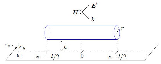
The first test setup in HIRF configuration consists of a PEC cylinder measuring l=5 m and r=1 m, situated in a height h=1 m above an infinitely extended ground plane, see Fig. 1. Hence, the conditions in a semi-anechoic chamber are tried to be approximated, which is the most common test site with regard to HIRF testing.

A linearly polarized plane wave characterized by an electrical field Eⁱ at a given frequency f is used as excitation. Propagation vector k heads in 45^∘-direction to the horizontal line, whereas magnetic field vector Hⁱ is tangential to the ground plane.

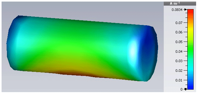
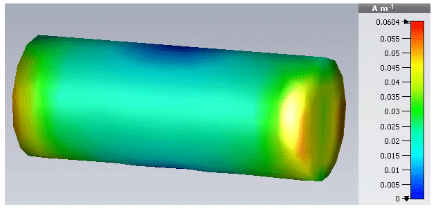
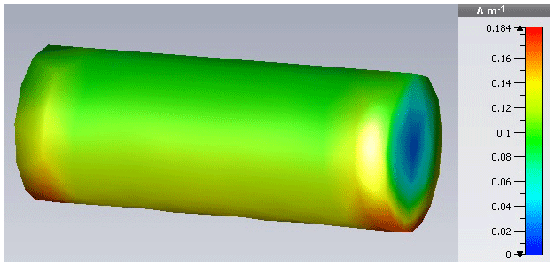
Initially, a CMA of the surface current is carried out using the integral equation solver of CST Microwave Studio resulting in the Characteristic HIRF Modes ${\mathit{J}}_n^{\text{H}},n=\mathrm{1},\mathrm{\dots },\mathrm{5}$ depicted in Figs. 2 to 6 as magnitude value. The triangular surface mesh used consists of n_t=402 triangles and n_p=223 grid points.

Figure 6 Characteristic Mode $\mathrm{|}{\mathit{J}}_{\mathrm{5}}^{\text{H}}\left(\mathit{r}\right)\mathrm{|}$ for f=f_res,1.

Each mode corresponds to a certain resonance of the system such as fundamental mode ${\mathit{J}}_{\mathrm{1}}^{\text{H}}$ and second harmonic ${\mathit{J}}_{\mathrm{2}}^{\text{H}}$, which indicate a λ∕2- and λ-resonance respectively.

The precise resonance frequencies of each mode are deduced from the modal significance s_n(f) illustrated in Fig. 7. Herein, only the fundamental mode shows a typical resonance-like curve with f_res,1≈20.7 MHz, whereas higher order modes either show no unique maximum or no maximum at all in the chosen frequency domain. One possible reason is a decreased quality factor due to radiation losses.

Figure 7 Modal significance s_n(f).

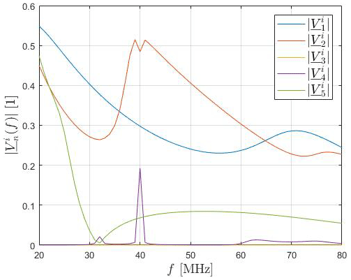
Figure 8 illustrates the magnitude of the modal excitation coefficients ${\underset{\mathrm{¯}}{V}}_n^i\left(f\right)$ numerically determined using FEKO, since CST does not provide these quantities. As can be seen, only the first two modes exhibit a relevant excitation throughout the entire frequency range.

Figure 8 Modal excitation coefficients $\mathrm{|}{\underset{\mathrm{¯}}{V}}_n^i\left(f\right)\mathrm{|}$.

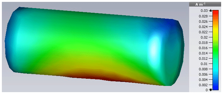
After the cylinder in HIRF-configuration has been analyzed by CMA, an exemplary excitation at f=40 MHz with |Eⁱ|=1 V m⁻¹ according to the model in Fig. 1 is investigated. The frequency was chosen such that no single Characteristic Mode dominates over others.

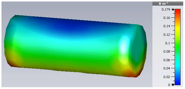
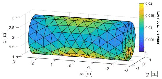
Then, the HIRF current ${\underset{\mathrm{¯}}{\mathit{J}}}_{\text{HIRF}}\left(\mathit{r}\right)$ on the cylinder arranges like in Fig. 9. Apparently, the current density is highest in the two bottom parts to the right and left, accompanied by a minimum close to the center.

Figure 9 HIRF current $\mathrm{|}{\underset{\mathrm{¯}}{\mathit{J}}}_{\text{HIRF}}\left(\mathit{r}\right)\mathrm{|}$ for f=40 MHz.

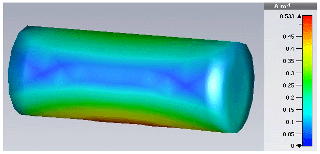
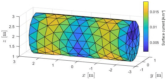
Taking the discussed results of CMA, it is possible to expand the total surface current of the preceeding HIRF excitation in terms of Characteristic Modes. Figure 10 outlines the associated Fourier series

$$\begin{array}{}\text{(8)}& \begin{array}{rl}& {\underset{\mathrm{¯}}{\mathit{J}}}_{\text{HIRF}}\left(\mathit{r}\right)\approx \sum _{n=\mathrm{1}}^N{\underset{\mathrm{¯}}{\mathit{\alpha }}}_n{\mathit{J}}_n^{\text{H}}\left(\mathit{r}\right)=\left(\mathrm{0.07}+\mathrm{j}\mathrm{0.28}\right){\mathit{J}}_{\mathrm{1}}^{\text{H}}\\ & +\left(\mathrm{0.20}+\mathrm{j}\mathrm{0.24}\right){\mathit{J}}_{\mathrm{2}}^{\text{H}}+\left(\mathrm{1.3}\times {\mathrm{10}}^{-\mathrm{5}}-\mathrm{j}\mathrm{2.9}\times {\mathrm{10}}^{-\mathrm{5}}\right){\mathit{J}}_{\mathrm{3}}^{\text{H}}\\ & -\left(\mathrm{0.08}+\mathrm{j}\mathrm{0.10}\right){\mathit{J}}_{\mathrm{4}}^{\text{H}}-\left(\mathrm{3.6}\times {\mathrm{10}}^{-\mathrm{3}}+\mathrm{j}\mathrm{1.9}\times {\mathrm{10}}^{-\mathrm{4}}\right){\mathit{J}}_{\mathrm{5}}^{\text{H}}\end{array}\end{array}$$

after Eq. (3) taking into account only N=5 modes. Although a non-resonance frequency was used as excitation, only three Characteristic Modes have significant influence on the total current. Distribution as well as amplitude fit the HIRF current to an acceptable degree except for the top left cylinder area. Raising the number of modes up to N=15 could not eliminate this circumstance, however, all other maxima could be reproduced.

Figure 10 Fourier series of $\mathrm{|}{\underset{\mathrm{¯}}{\mathit{J}}}_{\text{HIRF}}\left(\mathit{r}\right)\mathrm{|}$ for N=5 and f=40 MHz.

Since it is intended to approximate HIRF- by DCI-excitations, a comparison to a DCI setup's surface current is desirable. As test frequency serves the cylinder's first resonance obtained by CMA, which occurs at f_res,1=20.7 MHz correspondent to Fig. 7. Like Fig. 11 points out, the HIRF current ${\underset{\mathrm{¯}}{\mathit{J}}}_{\text{HIRF}}\left(\mathit{r}\right)$ accumulates at the bottom with a slight deviation from the center to the right.

Figure 11 HIRF current $\mathrm{|}{\underset{\mathrm{¯}}{\mathit{J}}}_{\text{HIRF}}\left(\mathit{r}\right)\mathrm{|}$ for f=f_res,1.

Figure 12 Fourier series of $\mathrm{|}{\underset{\mathrm{¯}}{\mathit{J}}}_{\text{HIRF}}\left(\mathit{r}\right)\mathrm{|}$ for N=5 and f=f_res,1.

Figure 13 DCI current $\mathrm{|}{\underset{\mathrm{¯}}{\mathit{J}}}_{\text{DCI}}\left(\mathit{r}\right)\mathrm{|}$ for f=f_res,1.

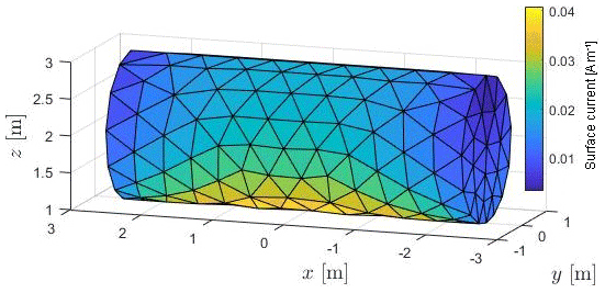
The way the HIRF current is composed of single Characteristic Modes is revealed by the series expansion

$$\begin{array}{}\text{(9)}& \begin{array}{rl}& {\underset{\mathrm{¯}}{\mathit{J}}}_{\text{HIRF}}\left(\mathit{r}\right)\approx \sum _{n=\mathrm{1}}^N{\underset{\mathrm{¯}}{\mathit{\alpha }}}_n{\mathit{J}}_n^{\text{H}}\left(\mathit{r}\right)=\left(\mathrm{0.19}-\mathrm{j}\mathrm{0.47}\right){\mathit{J}}_{\mathrm{1}}^{\text{H}}\\ & -\left(\mathrm{0.20}+\mathrm{j}\mathrm{0.10}\right){\mathit{J}}_{\mathrm{2}}^{\text{H}}-\left(\mathrm{7.3}\times {\mathrm{10}}^{-\mathrm{6}}-\mathrm{j}\mathrm{3.1}\times {\mathrm{10}}^{-\mathrm{6}}\right){\mathit{J}}_{\mathrm{3}}^{\text{H}}\\ & -\left(\mathrm{1.1}\times {\mathrm{10}}^{-\mathrm{7}}-\mathrm{j}\mathrm{7.6}\times {\mathrm{10}}^{-\mathrm{6}}\right){\mathit{J}}_{\mathrm{4}}^{\text{H}}-\left(\mathrm{0.02}-\mathrm{j}\mathrm{5.7}\times {\mathrm{10}}^{-\mathrm{4}}\right){\mathit{J}}_{\mathrm{5}}^{\text{H}}\end{array}\end{array}$$

showing a dominant fundamental mode, because its resonance frequency is used as excitation, but also a certain contribution of the second harmonic. Figure 12 stresses the aforementioned statement with a distribution looking similar to Characteristic Mode ${\mathit{J}}_{\mathrm{1}}^{\text{H}}$ in Fig. 2.

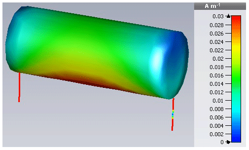
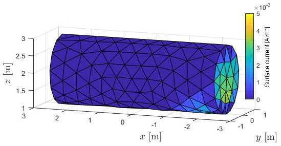
A DCI-configuration is specified by galvanically connecting both cylinder ends to the ground plane via two wire-shaped adapters. If the left one acts as excitation source with 50 Ω internal resistance and a power of 1 W at f=f_res,1 and the right one as termination with a 1 MΩ resistance, the resulting DCI current ${\underset{\mathrm{¯}}{\mathit{J}}}_{\text{DCI}}\left(\mathit{r}\right)$ distributes like in Fig. 13.

Figure 14 Fourier series of $\mathrm{|}{\underset{\mathrm{¯}}{\mathit{J}}}_{\text{DCI}}\left(\mathit{r}\right)\mathrm{|}$ for N=5 and f=f_res,1.

Figure 15 Absolute error ε(r_i) of HIRF and DCI for f=f_res,1.

Its decomposition into Characteristic DCI Modes ${\mathit{J}}_n^{\text{D}}$ is outlined by the corresponding series expansion

$$\begin{array}{}\text{(10)}& \begin{array}{rl}& {\underset{\mathrm{¯}}{\mathit{J}}}_{\text{DCI}}\left(\mathit{r}\right)\approx \sum _{n=\mathrm{1}}^N{\underset{\mathrm{¯}}{\mathit{\alpha }}}_n{\mathit{J}}_n^{\text{D}}\left(\mathit{r}\right)=\left(-\mathrm{0.06}+\mathrm{j}\mathrm{0.16}\right){\mathit{J}}_{\mathrm{1}}^{\text{D}}\\ & -\left(\mathrm{0.02}-\mathrm{j}\mathrm{0.11}\right){\mathit{J}}_{\mathrm{2}}^{\text{D}}+\left(\mathrm{1.6}\times {\mathrm{10}}^{-\mathrm{6}}-\mathrm{j}\mathrm{2.3}\times {\mathrm{10}}^{-\mathrm{5}}\right){\mathit{J}}_{\mathrm{3}}^{\text{D}}\\ & -\left(\mathrm{8.9}\times {\mathrm{10}}^{-\mathrm{6}}+\mathrm{j}\mathrm{1.9}\times {\mathrm{10}}^{-\mathrm{4}}\right){\mathit{J}}_{\mathrm{4}}^{\text{D}}-\left(\mathrm{1.6}\times {\mathrm{10}}^{-\mathrm{5}}-\mathrm{j}\mathrm{6.4}\times {\mathrm{10}}^{-\mathrm{4}}\right){\mathit{J}}_{\mathrm{5}}^{\text{D}}\end{array}\end{array}$$

depicted in Fig. 14 for the cylinder without its adapters. The attained coincidence in space and magnitude appears different. This is explainable with the fact that the DCI setup is not excited at its own resonance frequency, but with the HIRF setup's one. Consequently, the DCI fundamental mode is of decreased influence for the total DCI current.

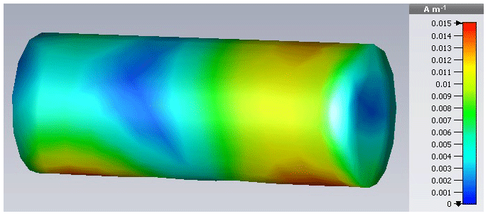
A quantitative comparison of HIRF and DCI is possible, when both currents are subtracted from each other at corresponding triangles located at ${\mathit{r}}_i,i=\mathrm{1},\mathrm{\dots },n_{\text{t}}$ of the simulation mesh yielding their absolute error

$$\begin{array}{}\text{(11)}& \mathit{\epsilon }\left({\mathit{r}}_i\right)=\left|{\underset{\mathrm{¯}}{\mathit{J}}}_{\text{HIRF}}\left({\mathit{r}}_i\right)-{\underset{\mathrm{¯}}{\mathit{J}}}_{\text{DCI}}\left({\mathit{r}}_i\right)\right|,\end{array}$$

whose graphical representation is given in Fig. 15. Apart from a small residual current at the right cylinder face its approximation to HIRF seems satisfying.

Figure 16 Characteristic Mode $\mathrm{|}{\mathit{J}}_{\mathrm{1}}^{\text{H}}\left(\mathit{r}\right)\mathrm{|}$ for f=f_res,1.

Figure 17 Characteristic Mode $\mathrm{|}{\mathit{J}}_{\mathrm{2}}^{\text{H}}\left(\mathit{r}\right)\mathrm{|}$ for f=f_res,1.

Figure 18 Characteristic Mode $\mathrm{|}{\mathit{J}}_{\mathrm{3}}^{\text{H}}\left(\mathit{r}\right)\mathrm{|}$ for f=f_res,1.

Figure 19 Characteristic Mode $\mathrm{|}{\mathit{J}}_{\mathrm{4}}^{\text{H}}\left(\mathit{r}\right)\mathrm{|}$ for f=f_res,1.

4 Car model

As more complex three-dimensional object a PEC car body is investigated. Its length is approximately 4 m with a maximum height of 1 m. The HIRF setup is geometrically the same as presented in Fig. 1, only with the DUT having been exchanged.

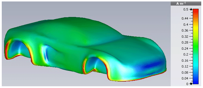
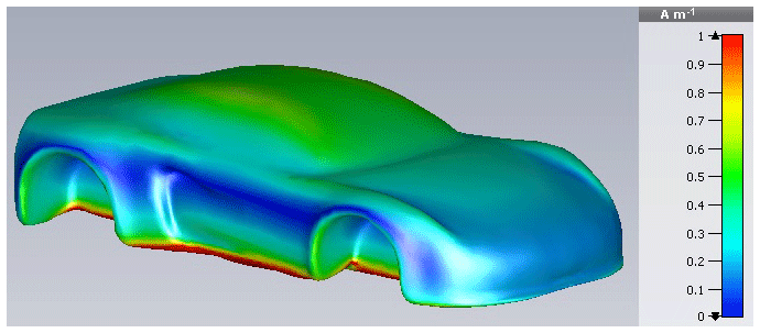
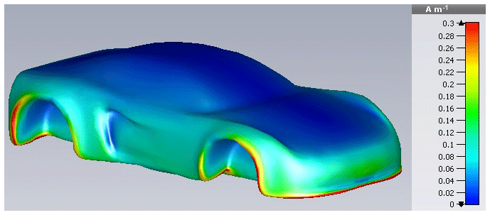
Given these preconditions, a CMA is processed for the first five surface current modes ${\mathit{J}}_n^{\text{H}}$, whose magnitude is illustrated in Figs. 16 to 20. Similar to the cylinder, basic resonance patterns such as half-, full- and higher-wave resonances can be observed by analyzing maxima and minima of the surface current. The triangular surface mesh used for all following simulations consists of n_t=12 412 triangles and n_p=6208 grid points.

Figure 20 Characteristic Mode $\mathrm{|}{\mathit{J}}_{\mathrm{5}}^{\text{H}}\left(\mathit{r}\right)\mathrm{|}$ for f=f_res,1.

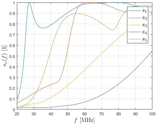
Surprisingly, the modal significance s_n calculated is comparable to those of the cylinder in Fig. 7, like Fig. 21 conveys. As an example, the first two harmonics basically have the same qualitative shape, but exhibit a frequency shift to slightly higher frequencies. This is due to the fact that the car is geometrically shorter implying higher resonance frequencies. Consequently, it can be stated that both test objects have similar electromagnetic properties regarding their frequency behavior, although being geometrically distinct. The fundamental mode's resonance frequency is $f_{\text{res},\mathrm{1}}\approx \mathrm{27.32}$ MHz, whereas higher harmonics do not expose a dedicated resonance frequency, as already noted for the cylinder.

Figure 21 Modal significance s_n(f).

Likewise, the modal excitation coefficients ${\underset{\mathrm{¯}}{V}}_n^i$ of the first couple of modes, see Fig. 22, appear to be comparable to their cylinder equivalents in Fig. 8, apart from the frequency shift already discussed for the modal significance. Again, the first two modes are excited most and, additionally, ${\mathit{J}}_{\mathrm{4}}^{\text{H}}$ also has a broadbanded influence on the total surface current. Nevertheless, the second mode is excited less at most frequency points compared to the cylinder implying a smaller Fourier coefficient ${\underset{\mathrm{¯}}{\mathit{\alpha }}}_{\mathrm{2}}$.

Figure 22 Modal excitation coefficients $\mathrm{|}{\underset{\mathrm{¯}}{V}}_n^i\left(f\right)\mathrm{|}$.

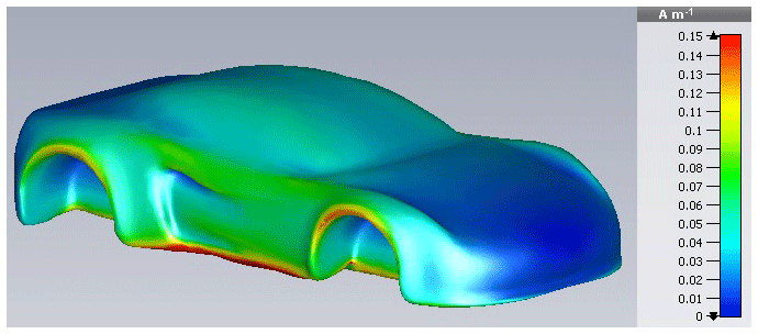
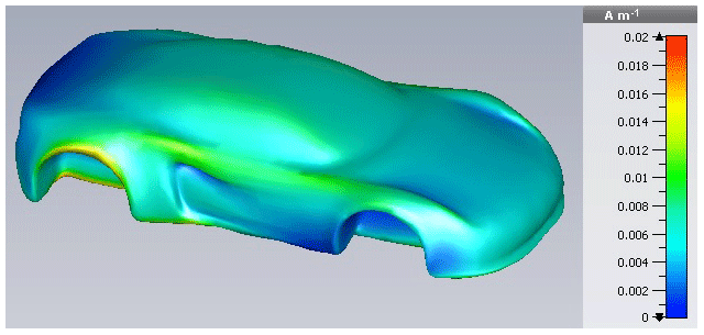
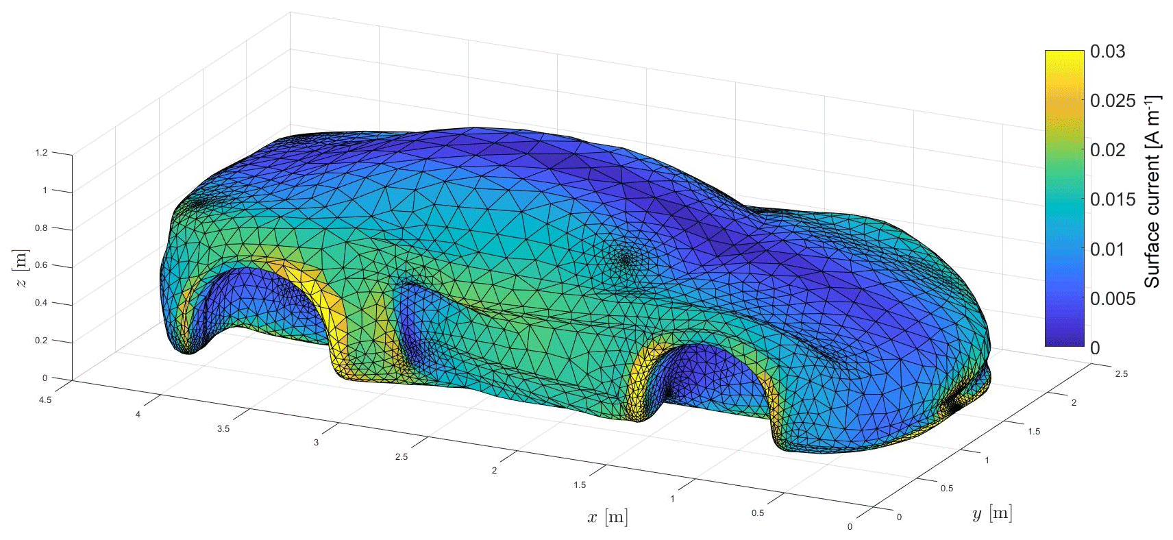
Once again, an attempt to expand the total surface current in Characteristic Modes is made. Herefore, the car is excited identically to the cylinder, i.e. with the same electrical field strength and frequency, the latter being selected intentionally different from a resonance. The resulting surface current, see Fig. 23, exposes a maximum in the rear wheel region, which should be reproduced because of its potential EMC relevance.

Figure 23 HIRF current $\mathrm{|}{\underset{\mathrm{¯}}{\mathit{J}}}_{\text{HIRF}}\left(\mathit{r}\right)\mathrm{|}$ for f=40 MHz.

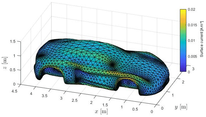
With the help of the modal excitation coefficients preceedingly discussed the desired Fourier series is set up to

$$\begin{array}{}\text{(12)}& \begin{array}{rl}& {\underset{\mathrm{¯}}{\mathit{J}}}_{\text{HIRF}}\left(\mathit{r}\right)\approx \sum _{n=\mathrm{1}}^N{\underset{\mathrm{¯}}{\mathit{\alpha }}}_n{\mathit{J}}_n^{\text{H}}\left(\mathit{r}\right)=\left(-\mathrm{0.22}+\mathrm{j}\mathrm{0.10}\right){\mathit{J}}_{\mathrm{1}}^{\text{H}}\\ & -\left(\mathrm{0.05}-\mathrm{j}\mathrm{3.1}\times {\mathrm{10}}^{-\mathrm{3}}\right){\mathit{J}}_{\mathrm{2}}^{\text{H}}+\left(\mathrm{4.1}\times {\mathrm{10}}^{-\mathrm{6}}+\mathrm{j}\mathrm{1.3}\times {\mathrm{10}}^{-\mathrm{6}}\right){\mathit{J}}_{\mathrm{3}}^{\text{H}}\\ & +\left(\mathrm{2.4}\times {\mathrm{10}}^{-\mathrm{3}}+\mathrm{j}\mathrm{1.5}\times {\mathrm{10}}^{-\mathrm{3}}\right){\mathit{J}}_{\mathrm{4}}^{\text{H}}-\left(\mathrm{1.8}\times {\mathrm{10}}^{-\mathrm{5}}-\mathrm{j}\mathrm{2.7}\times {\mathrm{10}}^{-\mathrm{5}}\right){\mathit{J}}_{\mathrm{5}}^{\text{H}}\end{array}\end{array}$$

using just five summands. It reveals larger errors in contrast to the cylinder expansion as depicted in Fig. 24. Beside the maximum in the rear wheel region, a further unintended maximum is generated at the front wheels. Apart from this region the current is quantitatively reproduced well by the series expansion. A possible explanation concerning the existing deviations is the larger complexity of the car's geometry such as the edges at which field excesses arise, which are more difficult to approximate.

Figure 24 Fourier series of $\mathrm{|}{\underset{\mathrm{¯}}{\mathit{J}}}_{\text{HIRF}}\left(\mathit{r}\right)\mathrm{|}$ for N=5 and f=40 MHz.

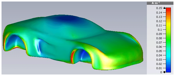
An equivalence consideration between HIRF and DCI is initiated by a field excitation with the car's first resonance frequency f_res,1, its result being illustrated in Fig. 25. The surface current ${\underset{\mathrm{¯}}{\mathit{J}}}_{\text{HIRF}}\left(\mathit{r}\right)$ is dominated by Characteristic Mode ${\mathit{J}}_{\mathrm{1}}^{\text{H}}$ because of a lack in significance of higher harmonics at this frequency.

Figure 25 HIRF current $\mathrm{|}{\underset{\mathrm{¯}}{\mathit{J}}}_{\text{HIRF}}\left(\mathit{r}\right)\mathrm{|}$ for f=f_res,1.

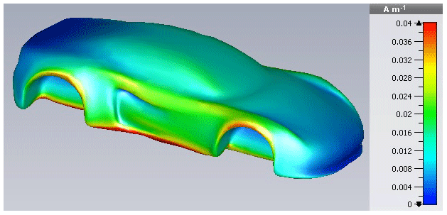
This is also supported by the series expansion in Characteristic Modes resulting in

$$\begin{array}{}\text{(13)}& \begin{array}{rl}& {\underset{\mathrm{¯}}{\mathit{J}}}_{\text{HIRF}}\left(\mathit{r}\right)\approx \sum _{n=\mathrm{1}}^N{\underset{\mathrm{¯}}{\mathit{\alpha }}}_n{\mathit{J}}_n^{\text{H}}\left(\mathit{r}\right)=\left(-\mathrm{0.31}-\mathrm{j}\mathrm{0.29}\right){\mathit{J}}_{\mathrm{1}}^{\text{H}}\\ & +\left(\mathrm{0.04}+\mathrm{j}\mathrm{0.02}\right){\mathit{J}}_{\mathrm{2}}^{\text{H}}-\left(\mathrm{5.7}\times {\mathrm{10}}^{-\mathrm{7}}-\mathrm{j}\mathrm{1.0}\times {\mathrm{10}}^{-\mathrm{6}}\right){\mathit{J}}_{\mathrm{3}}^{\text{H}}\\ & +\left(\mathrm{3.3}\times {\mathrm{10}}^{-\mathrm{3}}-\mathrm{j}\mathrm{5.6}\times {\mathrm{10}}^{-\mathrm{3}}\right){\mathit{J}}_{\mathrm{4}}^{\text{H}}-\left(\mathrm{2.1}\times {\mathrm{10}}^{-\mathrm{6}}-\mathrm{j}\mathrm{1.6}\times {\mathrm{10}}^{-\mathrm{6}}\right){\mathit{J}}_{\mathrm{5}}^{\text{H}}\end{array}\end{array}$$

from which the mentioned mathematical dominance of the first mode can been also seen in Fig. 26 when being compared to Characteristic Mode ${\mathit{J}}_{\mathrm{1}}^{\text{H}}$ in Fig. 16.

Figure 26 Fourier series of $\mathrm{|}{\underset{\mathrm{¯}}{\mathit{J}}}_{\text{HIRF}}\left(\mathit{r}\right)\mathrm{|}$ for N=5 and f=f_res,1.

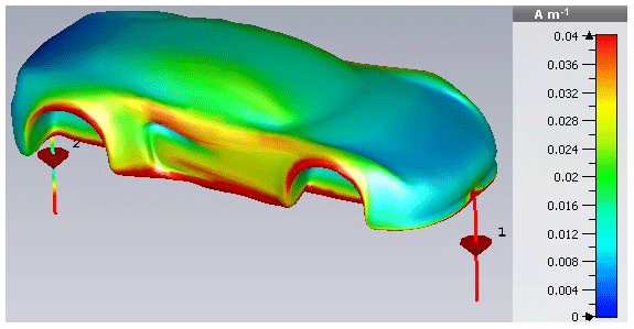
As DCI setup the same excitation scenario as with the cylinder is selected meaning a 50 Ω-source to the right and a high-impedance termination on the left hand side.

By visual comparison to the DCI current ${\underset{\mathrm{¯}}{\mathit{J}}}_{\text{DCI}}\left(\mathit{r}\right)$ in Fig. 27 an overtesting of the conducted setup can be noticed, e.g. at both wheels, but also in the area where the side doors are located.

Figure 27 DCI current $\mathrm{|}{\underset{\mathrm{¯}}{\mathit{J}}}_{\text{DCI}}\left(\mathit{r}\right)\mathrm{|}$ for f=f_res,1.

An expansion of the DCI-current in its affiliated Characteristic Modes gives

$$\begin{array}{}\text{(14)}& \begin{array}{rl}& {\underset{\mathrm{¯}}{\mathit{J}}}_{\text{DCI}}\left(\mathit{r}\right)\approx \sum _{n=\mathrm{1}}^N{\underset{\mathrm{¯}}{\mathit{\alpha }}}_n{\mathit{J}}_n^{\text{D}}\left(\mathit{r}\right)=\left(-\mathrm{0.06}+\mathrm{j}\mathrm{0.07}\right){\mathit{J}}_{\mathrm{1}}^{\text{D}}\\ & +\left(\mathrm{0.02}-\mathrm{j}\mathrm{0.03}\right){\mathit{J}}_{\mathrm{2}}^{\text{D}}-\left(\mathrm{7.6}\times {\mathrm{10}}^{-\mathrm{7}}+\mathrm{j}\mathrm{1.9}\times {\mathrm{10}}^{-\mathrm{6}}\right){\mathit{J}}_{\mathrm{3}}^{\text{D}}\\ & +\left(\mathrm{3.5}\times {\mathrm{10}}^{-\mathrm{3}}+\mathrm{j}\mathrm{7.8}\times {\mathrm{10}}^{-\mathrm{3}}\right){\mathit{J}}_{\mathrm{4}}^{\text{D}}+\left(\mathrm{2.6}\times {\mathrm{10}}^{-\mathrm{7}}+\mathrm{j}\mathrm{6.7}\times {\mathrm{10}}^{-\mathrm{7}}\right){\mathit{J}}_{\mathrm{5}}^{\text{D}}\end{array}\end{array}$$

with Fig. 28 as graphical representation. Just like in the cylinder's case, the first two Characteristic Modes contribute most to the total current. However, the current maxima at the wheels and the door are not equally reproduced.

Figure 28 Fourier series of $\mathrm{|}{\underset{\mathrm{¯}}{\mathit{J}}}_{\text{DCI}}\left(\mathit{r}\right)\mathrm{|}$ for N=5 and f=f_res,1.

Computing the absolute error ε(r_i) between HIRF- and DCI-excitation according to Eq. (11) followed by plotting the corresponding simulation mesh in Fig. 29 allows a numerical comparison. Unlike in the cylinder's case, a reasonable coincidence cannot be achieved. There still exists a significant surface current especially at the front wheel section and the door area.

Figure 29 Absolute error ϵ(r_i) of HIRF and DCI for f=f_res,1.

Table 1 additionally lists the absolute values $\mathrm{|}{\underset{\mathrm{¯}}{\mathit{\alpha }}}_n\mathrm{|}$ of all Fourier coefficients in Eqs. (8) to (10) and (12) to (14) allowing the contribution of single Characteristic Modes to be judged more clearly. Their order of magnitude directly indicates the degree of contribution to the total surface current despite a rather coarse truncation, which is of minor importance.

Table 1 Absolute values of the Fourier coefficients ${\underset{\mathrm{¯}}{\mathit{\alpha }}}_n$.

5 Conclusions

Characteristic Mode Analysis was introduced and applied to three-dimensional test objects. Based on computed Characteristic Modes for HIRF- and DCI-excitations, series expansions for surface currents were set up. Its coefficients gave a quantitative insight into the contribution of single Characteristic Modes to surface current distributions at different test frequencies. It could be shown for geometrically simple objects that HIRF excitations can be characterized by only a very limited number of Characteristic Modes both at resonance and beyond. Furthermore, CMA revealed geometrically different DUTs to be of comparable electrical characteristics due to similar modal significances, provided their overall dimensions coincide. Additionally, CMA turned out to be useful in finding resonance frequencies of complex systems, whose excitation is of relevance for EMC tests. Comparable HIRF and DCI excitations were given and a quantitative comparison of both current distributions was made based on absolute errors.