Analysis of large-scale UHF-RFID use-cases utilizing full-wave simulation techniques

UHF-RFID is a mature and widespread technology that has the potential to increase the reliability and efficiency of processes in logistics and production environments. However, complex interference effects in indoor environments pose challenges to the implementation of reliable wireless communication systems like RFID. This work proposes a method for tag performance evaluation utilizing a coherent two-stage rating process. This enables the abstraction of physical quantities and facilitates the interpretation of tag readability. For this purpose, two well-established full-wave techniques are utilized to perform deterministic simulations of a logistical UHF-RFID use-case. The setup of large-scale simulation environments is discussed and important quantities to be considered in RFID-systems are derived. Based on the simulation results and the proposed rating method, the RFID use-case is evaluated. Results are visualized in full-3D, facilitating the identification of critical spots. Furthermore, a subsequent cross-validation of the simulation results is performed, verifying the validity of the simulation results. By performing a priori propagation analysis, issues can effectively be revealed beforehand and costly modifications after system deployment can be avoided.

1 Introduction

Radio Frequency Identification (RFID) by now is a well-established technology throughout the whole supply chain. Many sub-processes, ranging from manufacturing and inventory management to transportation and distribution of goods, rely on RFID-systems to increase the degree of process transparency and automation, as well as the reliability and efficiency of the overall supply chain management. After more than a decade of ongoing research targeting various weak points (e.g. tag size, antenna and IC performance), modern systems offer optimal performance for a wide range of applications at low cost. This led to the comprehensive use of RFID.

Although RFID is a widely accepted and well-understood technology, challenges still persist. As the technology has the potential to tremendously increase reliability and efficiency, the sole implementation of this technology often leads to high expectations taking all potential benefits for granted. However, a successful and cost-optimal implementation of an RFID-system into a new environment requires a priori knowledge regarding the electromagnetic wave propagation. Analysis of indoor wave propagation comes with non-trivial challenges, e.g. interference effects in multipath environments, which are complex and hard to model. While early RFID-systems utilized the LF and HF frequency bands with very limited operational range, popular modern UHF-RFID-systems can operate up to 15 m (Finkenzeller and Müller, 2010), giving rise to strong multipath propagation. In addition, modern systems are used for more sophisticated tasks than just simple identification. Many processes in production rely on data saved on the tag IC or applications make use of Direction of Arrival (DoA) estimation to solve the task at hand (Ascher et al., 2017). Thus, the consequences of a system malfunction caused by interference can be severe, highlighting the necessity for sufficient propagation analysis. Further, a posteriori modification of the system and operational environment due to misbehaviour is very cost- and time-intensive. The ability to reveal issues already in the planning stage before system deployment is therefore highly desired.

Various approaches for signal coverage prediction exist, ranging from purely analytical and empirical (fast but inaccurate) to deterministic ones (higher computational effort but improved accuracy). Deterministic approaches include asymptotic methods, also often referred to as high frequency methods (e.g. Geometrical Optics and Physical Optics) and full-wave, or so-called low frequency methods (e.g. Finite Integration Technique, Finite Difference Time Domain, Method of Moments, Finite Element Method). Analysis of wave propagation in RFID-systems with analytical methods (Griffin and Durgin, 2009; Greene and Mickle, 2011; Bekkali et al., 2015), as well as asymptotic approaches (or a combination) have been widely studied in literature (Dimitriou et al., 2011; Bosselmann, 2010; Marrocco et al., 2009). Since most analytical methods are based on the free-space Friis transmission equation or use a combination of statistical models, complex effects like site-specific small-scale fading and multipath propagation can not be taken into account accurately or at all. While the asymptotic approach, especially if combined with improvements like Uniform Theory of Diffraction (UTD), can yield useful results for simple scenarios, the high frequency approximation for this method can introduce significant inaccuracies, in particular considering the relatively long wavelength of λ=34.5 cm for UHF-RFID (Bosselmann, 2010). Because of this, full-wave techniques that solve Maxwell's equations with no fundamental approximations are of high interest.

The analysis of UHF-RFID scenarios utilizing full-wave methods has only been reported for separate small-scale applications (Hoefinghoff et al., 2011). Since in recent years available computational resources increased and High Performance Computing (HPC) in combination with code parallelization gained popularity, full-wave analysis became more feasible. Deterministic analysis becomes more attractive as the availability of detailed virtual 3D models increases, and their utilization throughout the whole life cycle of physical products and whole environments like factories is prioritized (Grieves, 2015; Digitale Fabrikplanung AG, 2009). This process of creating a highly accurate virtual copy of the physical object is called digital twinning. The global research firm Gartner recently rated digital twinning as one of the top 10 disruptive technology trends for multiple years in a row (Gartner, 2018). In view of emerging technologies and the demanding requirements regarding industry 4.0 and industrial IoT, this trend is expected to be continued. In order to follow current technology trends utilizing their full potential and meeting the steadily growing requirements for modern communication systems, new methods with higher accuracy for signal propagation analysis in large realistic scenarios are required.

This work proposes a method for tag performance evaluation, based on results obtained from accurate full-wave simulations. A two-stage rating process is developed to abstract physical quantities and yield results that enable a convenient interpretation, including individuals without a strong technical background. The remaining of the paper is structured as follows. Section 2 gives an overview of popular full-wave methods and discusses the set-up of large-scale environments using selected simulation techniques. Section 3 focuses on result evaluation, applying the proposed method for tag readability rating on a logistical RFID use-case, followed by the validation of the simulation results.

Table 1 Overview of well-established full-wave techniques with details regarding their most common implementation.

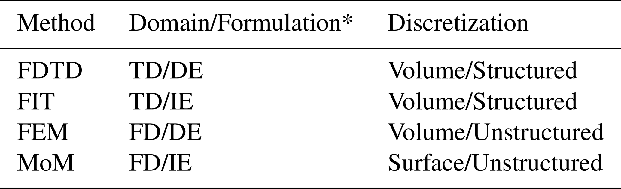
* TD/FD: Time/Frequency Domain | DE/IE: Differential/Integral Equation

2 Simulation methods and environment

Full-wave techniques belong to the field of computational electromagnetics (CEM). Their aim is to numerically solve the Maxwell's equations without any initial physical approximation (unlike asymptotic methods), so the vector nature of the electromagnetic field can be fully taken into account. Various full-wave techniques exist, some of which are widely studied and numerous efficient software implementations are available (see Table 1).

As computational resources are finite, the continuous electromagnetic field has to be adequately discretized. The discretization of the calculation domain, thus the subdivision of the full model into small parts (meshing), is fundamental to all methods. Solving for an unknown electromagnetic quantity, which depending on the utilized mesh can either be the electric and magnetic field (e.g. FIT, FDTD, FEM) or the surface currents (e.g. MoM), is the aim of the computations. The methods are often categorized based on the domain of operation (time or frequency domain), the form of the utilized Maxwell's equations (differential or integral form) or the kind of underlying discretization (structured/unstructured grid and surface/volume based mesh) (Davidson, 2010). Depending on the type and implementation of the method, there are different advantages and shortcomings to be taken into account, rendering the respective method more or less suited for a certain problem.

For the subsequent analysis, the two powerful and popular methods Finite Integration Technique (FIT) and Method of Moments (MoM) with its iterative implementation Multi-Level Fast Multipole Method (MLFMM) are utilized. Both methods are implemented in the commercially available CEM package CST Microwave Studio Suite, as the transient time domain solver (T-Solver) and the surface based integral equation solver (I-Solver) respectively.

The T-Solver uses a hexahedral mesh in cartesian coordinates, discretizing Maxwell's equations in integral form on staggered grids. The Maxwell's equations can be conveniently applied to the grid by using electric and magnetic voltages on mesh cell edges, related to the electric and magnetic fluxes through mesh cell faces. Explicit time-stepping is used (leap-frog-scheme) to propagate the fields through the calculation domain. Thus, field values of a subsequent time step can be calculated from fields at the current and previous time steps, leading to a sparse matrix-vector multiplication at each time step. In addition, using advanced techniques like the Perfect Boundary Approximation (PBA) it is possible to apply efficient meshing even for curved structures and overcome issues like the stair-stepping effect standard FDTD code suffers from. All in all, this makes the requirements in computation time and memory increase linearly with the number of mesh cells, enabling simulation of electrically large structures (Weiland, 1977).

The I-Solver uses a curved triangular surface mesh and surface currents to solve the problem at hand. After discretization of the surface integral formulation using Combined Field Integral Equation (CFIE), a matrix equation modelling the interactions between each surface element is set up. The MoM is used on the CFIE by expanding the surface currents with adequate basis functions according to the Galerkin method. This leads to a dense matrix equation system. Thus, using a direct solver approach, the computational effort and memory requirements become prohibitive fast. However, solving the system in an iterative manner using the Multi-Level Fast Multipole Method (MLFMM) enables large-scale computations. When applying the MLFMM, surface elements next to each other are clustered into groups. Subsequently, only the coupling between clusters is considered, approximating the coupling of individual elements to each other, enabling acceleration of the matrix-vector multiplication. However, this approximation is only valid if the clusters are sufficiently far away from each other. If this is not the case, the element couplings must be solved with the direct method. Thus, if MLFMM can be applied, the method scales with linear-logarithmic complexity 𝒪(nlog n) in time and memory (Davidson, 2010). As only the surface is meshed, this method is efficient for scenarios containing large areas of free space.

These solvers have been chosen as they potentially offer the possibility to tackle electrically large problems, as well as due to their fundamentally different mathematical core. This enables cross-validation of simulation results, as discussed in Sect. 3.3.

2.1 Set-up of the simulation environment

Detailed 3D CAD models are created during the planning stage of a logistical environment, to be imported into CST Microwave Studio for large-scale simulations. The models consist of solid bodies and are free of intersections to prevent meshing issues. The file format of the CAD models has to offer the possibility to differentiate between objects and components, so material properties relevant for the electromagnetic simulation can be properly assigned and taken into account respectively.

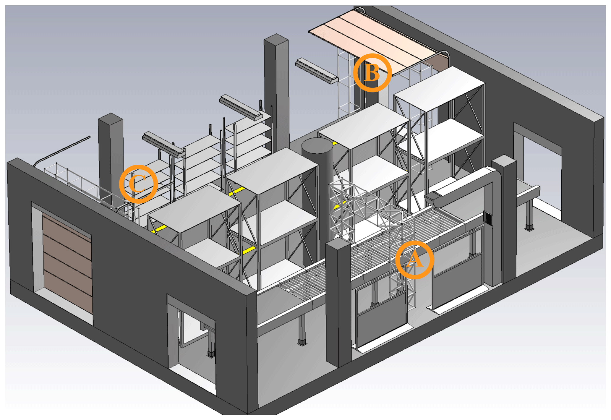
Figure 1 Analyzed model presented in side view. Three RFID gates are present in this scenario, marked with A, B and C respectively. The ceiling is included in the simulation as well, but hidden here for visualization's sake.

The model to be analyzed in this work is shown in Fig. 1. It is a common logistics environment, consisting of a conveyer belt with a small RFID gate to scan passing goods on the right (marked with A, antenna at the side of the gate) and two bigger RFID gates placed at the entrance (B, antenna on top of the gate) and at the exit (C, antenna on top). The left hand side of the hall represents a storage room. Goods are delivered by a forklift to the entrance and checked-in at RFID gate B, while leaving the storage room and checked-out at the exit at gate C. Gate A scans goods, moved to another subsequent storage room. Because multiple RFID-readers suiting different purposes are deployed, it is important to ensure that tagged goods can only be read by the intended RFID-reader (Sect. 3.2 covers this topic more in depth). Besides the obvious objects like storage racks and gates, also various details like ventilation shaft, room lighting, movable walls, dock doors etc. are modelled in the presented environment. The radiation emitted by the antenna at gate A and gate B is analyzed in this work. Figure 2 gives an overview of the scenario including its dimensions, with a width (W) of 10 m, length (L) of 14 m and a height of 4.90 m.

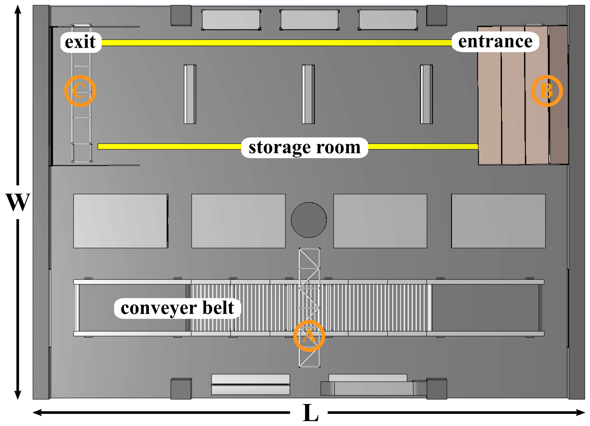
Figure 2 Analyzed model presented in bird's eye view. Width of the model is 10 m, length 14 m and height 4.90 m. Markings A, B and C show the positions of the antenna mountings for every gate.

2.1.1 Geometric model and meshing techniques

Before simulation launch, relevant electromagnetic material properties are assigned, and a discretization of the calculation domain is performed. To model a realistic environment, lossy dielectric materials exhibiting various permittivity values are utilized within the investigated scenario. In this work, all material properties are loaded from the material library in CST. For example, room structures (e.g. floor, walls) are modeled with concrete, parts of the conveyer belt with rubber and subcomponents of the room lighting and the movable walls consist of glass. All conductive materials, present in e.g. gates, conveyer framework, racks etc., are approximated with the Perfect Electric Conductor (PEC).

The accuracy of the simulation results strongly depends on the utilized mesh. Generally speaking, the finer the mesh, the higher the accuracy of the results. However, for large-scale simulations, applying a dense mesh or performing convergence studies becomes prohibitive. Thus, a considered compromise is necessary. When generating a mesh, two main factors have to be considered: sufficient resolution of the propagating wave, i.e. adequate sampling of phase information, and proper representation of the geometric structure.

The hexahedral mesh (T-Solver) is generated based on specified mesh cells per wavelength. This value is crucial as it dictates the memory and time requirements for the simulation, but also the resolution of phase sampling. To avoid significant phase errors, one wavelength should be resolved with at least 10 mesh cells. For differential equation solvers, where grids propagate the solution, a higher value is advisable to counter the effect of numerical dispersion (Rylander et al., 2012). Attention should be given to the smallest mesh cell in the scenario, as it determines the time step for the numerical wave propagation (Courant stability condition). In the subsequent simulations, if not stated otherwise, a value of 15 cells per wavelength is applied, what is a relatively dense mesh. To adequately resolve the geometric model, mesh snapping is applied to edges, planes and spheres.

While the hexahedral mesh in general can be applied “out of the box”, the meshing process for an unstructured grid, like the curved triangular surface mesh (I-Solver), is more complex. Imported models often can not be successfully meshed right away but manual adjustments are necessary. Intersections and gaps pose a problem and have to be fixed. The surface elements used by the I-Solver should exhibit a sufficient quality. Although preconditioning is performed for the matrix equations in the utilized simulation tool, it is vital to avoid low quality elements (large dihedral angles or large element edge-to-edge ratios). Poor quality elements lead to a worse condition number of the system matrix. This has a huge negative impact on the convergence of the system, thus the simulation time.

To accurately consider the interaction of the electromagnetic fields with dielectrics, the mesh should be refined based on materials. Mesh refinement at edges and detailed geometric structures improves the sampling of complex effects, however, large-scale simulations require mesh adaptations to decrease computational effort. Thus, improved mesh refinement is applied locally for areas with a high field presence (e.g. near to the source) and neglected for remaining areas. Open boundaries are applied, so electromagnetic waves leaving the calculation domain are absorbed. For this, a Perfectly Matched Layer (PML) is utilized. This is computationally intensive and leads to increased memory consumption. Whenever reasonable, calculation domain boundaries should be approximated, e.g. utilizing PEC walls.

2.1.2 Sources and excitation

The setup of accurate excitation sources is crucial to perform meaningful simulations. However, to sufficiently resolve all electrically meaningful details of a full antenna model, a high density mesh is required, rendering a full-wave simulation of a large-scale scenario unfeasible. Because of this, the actual antenna model is replaced with an equivalent source representation, called a Near-Field Source (NFS). This technique is commonly used in large simulations in the aviation and space field. A NFS is based on the field equivalence principle, which states that the fields outside an imaginary closed surface (Huygens' Box) can be obtained by imprinting equivalent electric and magnetic currents onto the imaginary boundary surface. The currents force the fields inside the closed surface to vanish and to be equivalent to the radiation produced by the actual source outside the Huygens' Box (Balanis, 2016).

The full antenna model is simulated in a separate small-part simulation, applying an adequate high density mesh. During this simulation the NFS is recorded and subsequently used as source in the large-scale simulation. This completely eliminates the high requirements to accurately resolve the electrically small details of the full antenna model. In addition, this enables the coupling of multiple simulations, using different simulation methods (hybrid approach), as well as accurate simulations of antennas without the full model available (e.g. vendors usually do not want to hand out detailed models of their products). A NFS can not only be created in a simulation, but also by near-field measurements (Foged et al., 2014).

Using equivalent source representations in form of a NFS as excitation is potentially very accurate. By simulating the full antenna including a part of its platform, the NFS is able to capture near-field coupling effects. This enables taking reciprocal effects of antenna and platform into account (Malmström et al., 2018). Figure 3 shows the simulation setup used for the NFS generation for the small RFID gate A. The NFS is recorded while simulating the full antenna model including a part of the antenna platform, depicted with a yellow box in (a). By comparing the cross-section of the electric-field distribution of the full antenna model (b) and the field distribution radiated by the NFS (c), equivalence can be confirmed. Figure 4 shows a polar plot containing far-field results of the electric-field in elevation plane including a part of the platform, radiated by the actual antenna structure and the NFS respectively.

For this simulation a circular patch antenna based on the design in Padhi et al. (2003) and adopted for the UHF-RFID 868 MHz band is used. Excitations are performed without modulation.

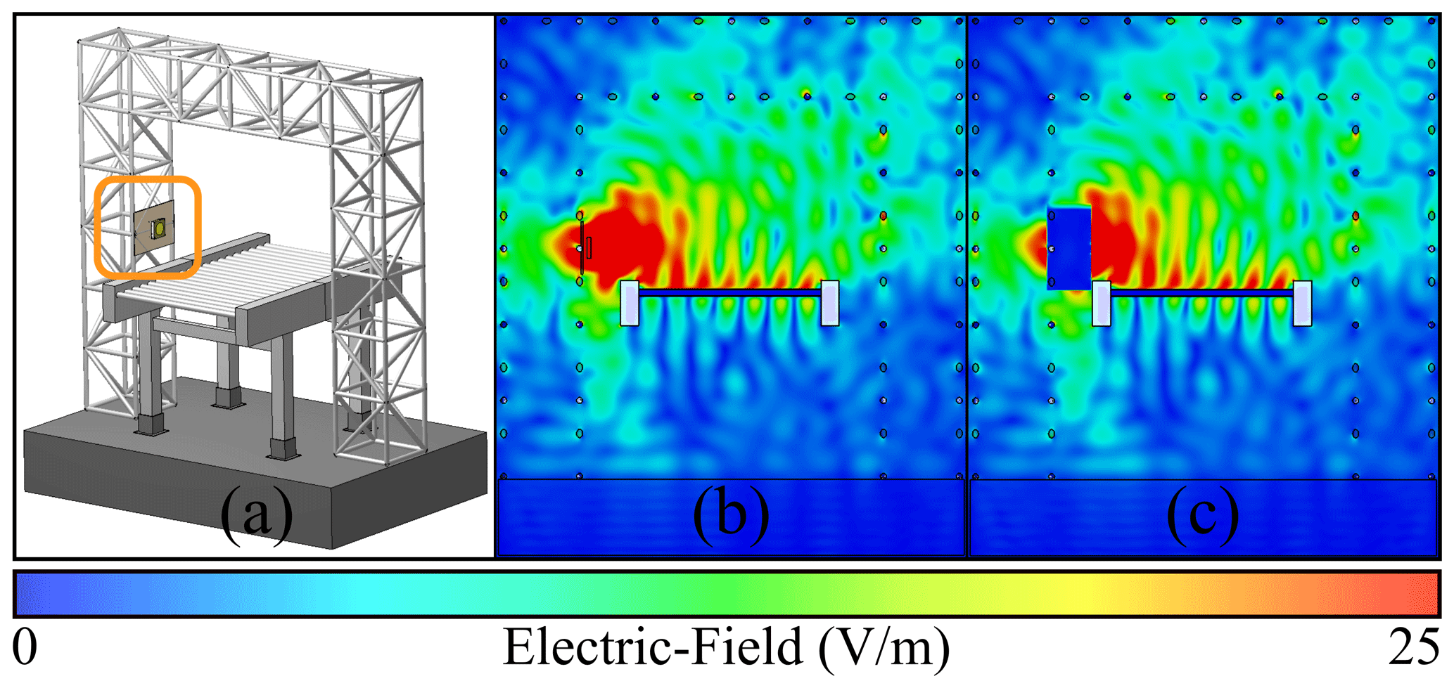
Figure 3 Gate A (platform) with the RFID-reader antenna attached (a), the electric-field distribution (cross-section) of the simulated full antenna model (b) and the field distribution for the simulation using the NFS as equivalent source (c). Yellow box in (a) depicts the volume used for NFS recording, including a part of the platform.

3 Evaluation of simulation results

This section covers the processing and evaluation of the simulation results. First, UHF-RFID brings some differences compared to other wireless communication systems. The RFID-reader communicates with the tag using backscattering, thus the power received by the tag is reflected back to the reader, modulated by changing impedance states (Finkenzeller and Müller, 2010). The sensitivity of modern RFID-reader devices (minimum power that can be detected) is far below the sensitivity of an RFID-tag, so as the communication channel is reciprocal, the reader will be able to communicate with the tag if enough power has been received by the tag to respond. Because of the narrowband nature of UHF-RFID and the limited operational range for passive backscattering systems, delay spread and Inter Symbol Interference (ISI) can be neglected. This by definition makes a flat communication channel, eliminating the necessity to consider frequency selective channel-fading. Thus, the evaluation in the following sections focuses on the physical layer (electromagnetic wave propagation) of the forward link (reader to tag), as this is usually the limiting factor in the communication chain of passive backscatter applications. The results are evaluated at a frequency of 868 MHz.

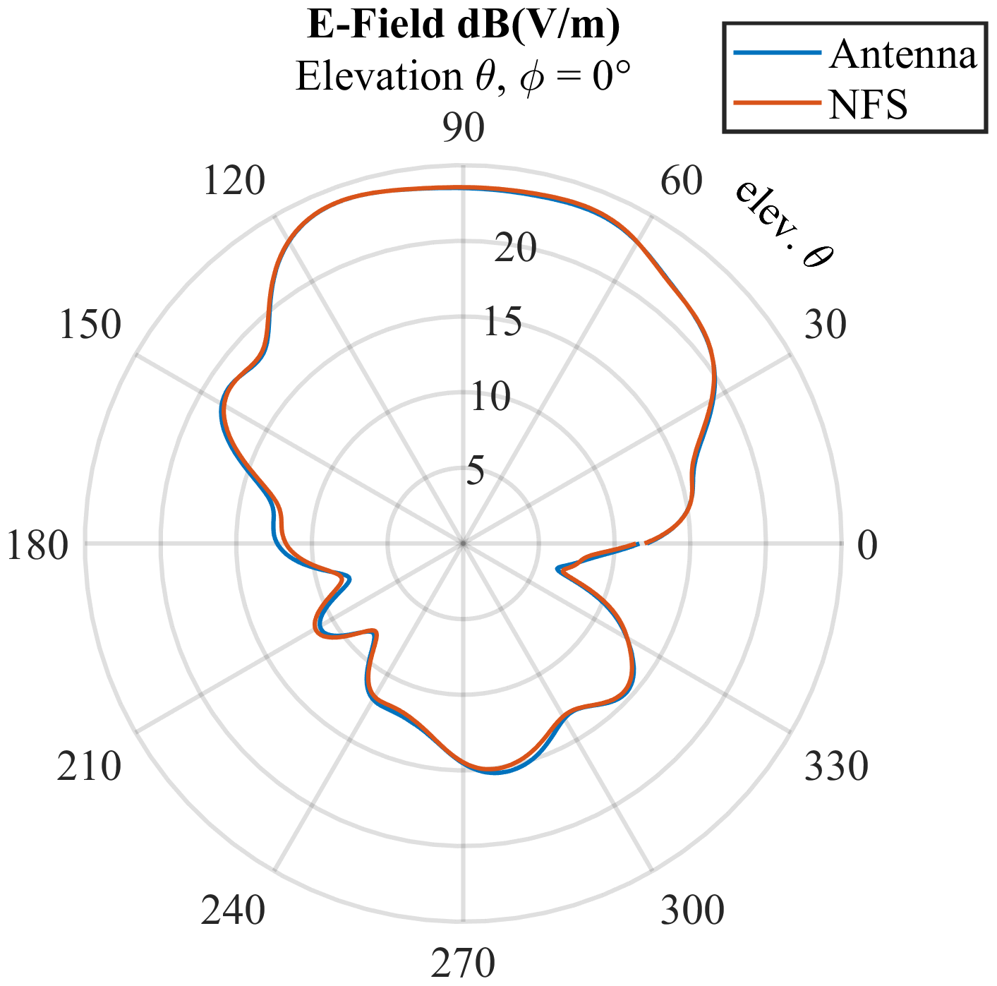
Figure 4 Electric far-field of the full antenna model and the NFS including a part of the platform in elevation plane respectively (elevation $\mathit{\theta },\mathrm{const}.\mathit{\varphi }=\mathrm{0}$^∘).

The simulation results used for the subsequent analysis consist of complex electric-field exports, to be used for the calculation of field strength and wave polarization, as well as power-flow exports to gain information regarding the propagation direction. The simulation results are imported and evaluated using a custom tool developed in Python. The spacing for the visualization and the following analysis is chosen to be uniformly cubic in 5 cm steps. This spacing has been found to be convincing for tag performance evaluation, as it compares well to most commonly used UHF-RFID-tag sizes, but still allows a fairly dense discretization to capture crucial fading effects in the environment.

3.1 Interpretation of readability

As the interpretation of tag performance solely based on the electric-field is quite ambiguous, other quantities enabling a meaningful interpretation need to be derived. The following section is dedicated to the derivation of adequate quantities to be used in a two-stage rating process to facilitate tag readability rating.

The amount of power received by an antenna P_tag is calculated by multiplying the effective antenna aperture A_eff by the power density of the incident wave S and the Polarization Loss Factor (PLF) m_plf:

$$\begin{array}{}\text{(1)}& P_{\mathrm{tag}}=S{A}_{\mathrm{eff}}{m}_{\mathrm{plf}}.\end{array}$$

The effective antenna aperture is given by

$$\begin{array}{}\text{(2)}& A_{\mathrm{eff}}={\displaystyle \frac{{\mathit{\lambda }}^{\mathrm{2}}}{\mathrm{4}\mathit{\pi }}}G\end{array}$$

for a specified antenna gain G (Balanis, 2016). Using the following equation to relate the RMS magnitude of the electric-field vector to the power density,

$$\begin{array}{}\text{(3)}& S={\displaystyle \frac{|E{|}^{\mathrm{2}}}{\mathrm{120}\mathit{\pi }}}\end{array}$$

yields the equation to compute the received power at the tag antenna:

$$\begin{array}{}\text{(4)}& P_{\mathrm{tag}}={\left({\displaystyle \frac{\mathit{\lambda }\left|E\right|}{\mathrm{4}\mathit{\pi }\sqrt{\mathrm{30}}}}\right)}^{\mathrm{2}}\cdot G\cdot m_{\mathrm{plf}}.\end{array}$$

Often in common RFID-system setups the PLF is considered to be 0.5 when using circularly polarized antennas at the reader side and linearly polarized tag antennas. However, the polarization of the emitted wave is not uniform, but strongly dependent on the angle to the emitting antenna. It is widely known that multipath interference, which is especially strong in indoor environments, has a significant impact on the polarization state of waves, and so does the interaction of propagating waves with the environment (Ippolito et al., 1989; Middlestead, 2017; Eschlwech and Biebl, 2018). Therefore, the PLF must be taken into account by calculation.

Figure 5 Tilted polarization ellipse with semi-major axis (OA) and semi-minor axis (OB).

The instantaneous field of an elliptically polarized plane wave (linearly and circularly polarized waves being the special cases of an elliptical wave) traveling in positive z direction is given by

$$\begin{array}{}\text{(5)}& E(t,z)=E_x(t,z)+E_y(t,z)\end{array}$$

with its decomposed orthogonal components and the field magnitudes of E_0x and E_0y respectively

$$\begin{array}{}\text{(6)}& {\displaystyle }{E}_x(t,z)=E_{\mathrm{0}x}\cos (\mathit{\omega }t-\mathit{\beta }z+{\mathit{\varphi }}_x)\text{(7)}& {\displaystyle }{E}_y(t,z)=E_{\mathrm{0}y}\cos (\mathit{\omega }t-\mathit{\beta }z+{\mathit{\varphi }}_y)\end{array}$$

with angular frequency ω, wavenumber β and their respective phases ϕ_x and ϕ_y. The phase difference between the components is given by

$$\begin{array}{}\text{(8)}& \mathrm{\Delta }\mathit{\varphi }={\mathit{\varphi }}_y-{\mathit{\varphi }}_x.\end{array}$$

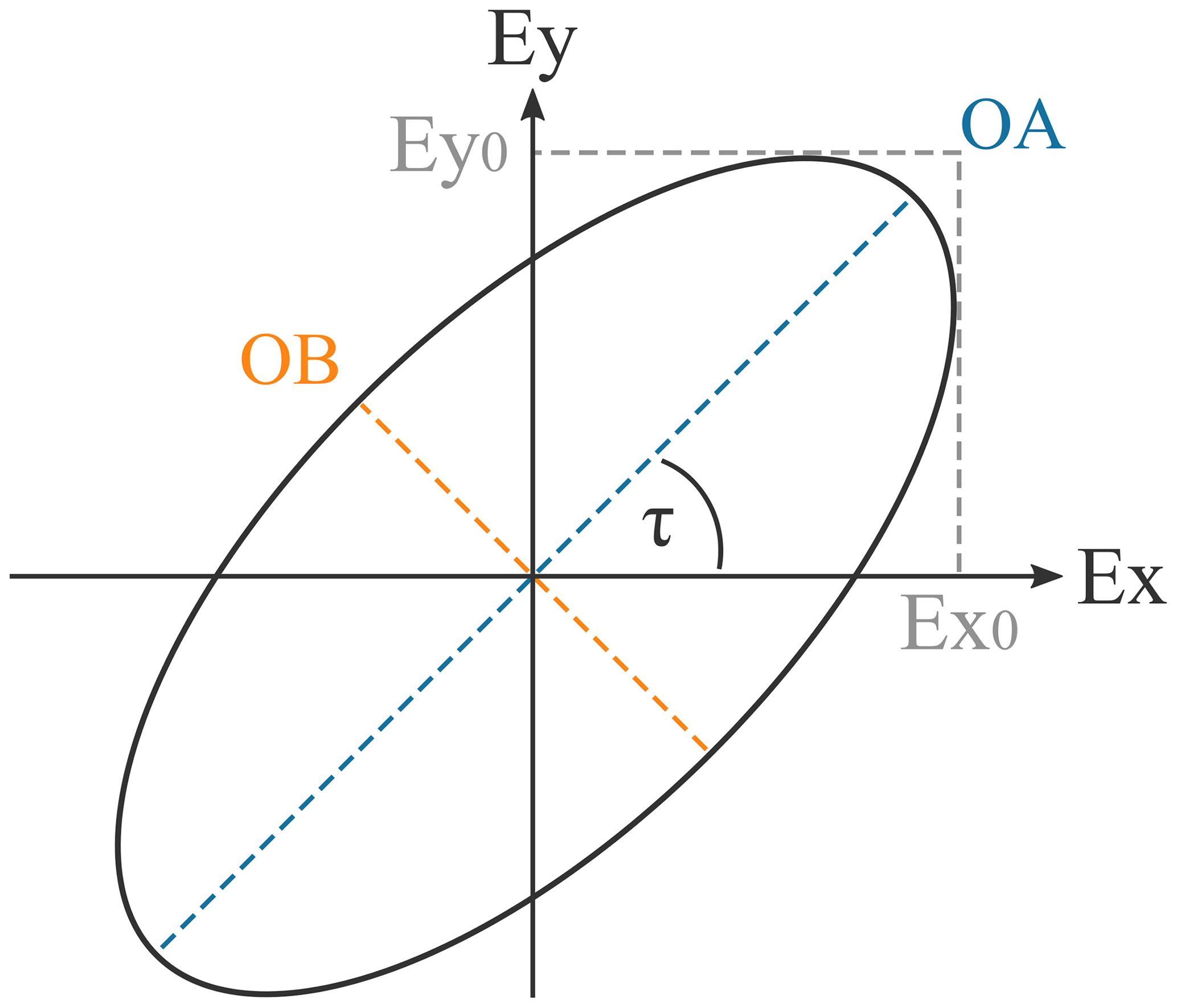
Using the magnitudes of the orthogonal parts and the relative phase shift, the semi-major axis (OA) and semi-minor axis (OB) of the polarization ellipse (see Fig. 5) traced out by the rotating field vector can be calculated with

$$\begin{array}{}\text{(9)}& {\displaystyle }\mathrm{OA}=\sqrt{{\displaystyle \frac{E_{x\mathrm{0}}^{\mathrm{2}}+E_{y\mathrm{0}}^{\mathrm{2}}+\sqrt{E_{x\mathrm{0}}^{\mathrm{4}}+E_{y\mathrm{0}}^{\mathrm{4}}+\mathrm{2}{E}_{x\mathrm{0}}^{\mathrm{2}}{E}_{y\mathrm{0}}^{\mathrm{2}}\cos \left(\mathrm{2}\mathrm{\Delta }\mathit{\varphi }\right)}}{\mathrm{2}}}},\text{(10)}& {\displaystyle }\mathrm{OB}=\sqrt{{\displaystyle \frac{E_{x\mathrm{0}}^{\mathrm{2}}+E_{y\mathrm{0}}^{\mathrm{2}}-\sqrt{E_{x\mathrm{0}}^{\mathrm{4}}+E_{y\mathrm{0}}^{\mathrm{4}}+\mathrm{2}{E}_{x\mathrm{0}}^{\mathrm{2}}{E}_{y\mathrm{0}}^{\mathrm{2}}\cos \left(\mathrm{2}\mathrm{\Delta }\mathit{\varphi }\right)}}{\mathrm{2}}}}\end{array}$$

respectively (Balanis, 2016). The ratio of the two axes of the polarization ellipse yields the axial ratio (AR) of the propagating wave:

$$\begin{array}{}\text{(11)}& \mathrm{AR}={\displaystyle \frac{\text{major axis}}{\text{minor axis}}}={\displaystyle \frac{\mathrm{OA}}{\mathrm{OB}}},\mathrm{0}\le \mathrm{AR}\le \mathrm{\infty }.\end{array}$$

Further, the PLF for the general case is given by

$$\begin{array}{}\text{(12)}& m_{\mathrm{plf}}={\displaystyle \frac{\mathrm{1}}{\mathrm{2}}}+{\displaystyle \frac{\mathrm{4}{r}_{\mathrm{w}}{r}_{\mathrm{a}}+(r_{\mathrm{w}}^{\mathrm{2}}-\mathrm{1})(r_{\mathrm{a}}^{\mathrm{2}}-\mathrm{1})\cos \left(\mathrm{2}\right({\mathit{\tau }}_{\mathrm{a}}-{\mathit{\tau }}_{\mathrm{w}}\left)\right)}{\mathrm{2}(r_{\mathrm{w}}^{\mathrm{2}}+\mathrm{1})(r_{\mathrm{a}}^{\mathrm{2}}+\mathrm{1})}}\end{array}$$

with r_w being the AR of the impinging wave and r_a the polarization state of the receiving antenna (Ippolito et al., 1989). The angular difference $\mathrm{\Delta }\mathit{\tau }={\mathit{\tau }}_{\mathrm{a}}-{\mathit{\tau }}_{\mathrm{w}}$ specifies the offset, thus the misalignment of the two major-axes of the polarization ellipses to each other. Depending on the degree of mismatch, the PLF lies in the range $\mathrm{0}\le m_{\mathrm{plf}}\le \mathrm{1}$ (m_plf=0 implies maximal loss, i.e. orthogonal misalignment, and m_plf=1 no loss, i.e. parallel alignment). As RFID-tag antennas are linearly polarized, the formula for the present case simplifies to (AR for linear polarization is assumed r_a=∞, thus in the following r_w=r)

$$\begin{array}{}\text{(13)}& m_{\mathrm{plf}}={\displaystyle \frac{\mathrm{1}}{\mathrm{2}}}+{\displaystyle \frac{(r^{\mathrm{2}}-\mathrm{1})\cos \left(\mathrm{2}\mathrm{\Delta }\mathit{\tau }\right)}{\mathrm{2}(r^{\mathrm{2}}+\mathrm{1})}},\mathrm{0}\le m_{\mathrm{plf}}\le \mathrm{1}.\end{array}$$

To highlight the necessity for these calculations, considering an elliptically polarized wave and a linear antenna, an AR of r=2 already leads to a PLF ranging from 0.2 to 0.8, depending on the orientation of the polarization ellipse to the antenna (Ippolito et al., 1989).

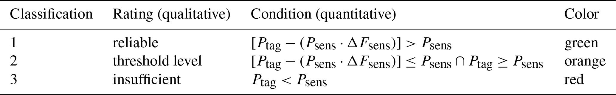
Table 2 Stage I readability rating: Defined categories with natural language descriptors and their respective condition.

The tag performance evaluation in the following is based on the power received by the tag antenna deliverable to the load P_tag, in relation to the sensitivity value P_sens of the tag IC. To facilitate the evaluation, a two-stage rating process is proposed.

In stage I, the rating is based on the delivered power, according to Eq. (4), considering the computed polarization ellipse under ideal alignment. Tag locations are classified into three groups: reliable (tag can be read), threshold level (readability potentially unreliable) and insufficient (tag cannot be read). Additionally, a factor ΔF_sens is introduced to define the width of the threshold level class and adjust its margin. This makes it possible to introduce a buffer as a function of the sensitivity value to counter uncertainty. Table 2 gives an overview of the defined rating classes and their respective conditions.

Stage II of the rating process determines the final readability rating, taking all possible polarization states into account. Analysis in this stage only considers tag locations that have been classified as reliable in the previous rating phase, all other tag locations are rated with zero percent readability. Recalling Fig. 5, it is obvious that the polarization ellipse can be rotated by 360^∘. However, as all four quadrants yield equal results, the rotation range reduces to 90^∘. By rotating the computed polarization ellipse in one degree steps, all rotation states are evaluated regarding the amount of received power according to Eq. (4) respectively. Alignments that yield sufficient power for the given tag location are counted. Thus, with total states to be evaluated T_total=90, and the count of states that deliver sufficient power T_read, Eq. (14) yields the total readability R_tag for the given tag location in percent:

$$\begin{array}{}\text{(14)}& R_{\mathrm{tag}}={\displaystyle \frac{T_{\mathrm{read}}}{T_{\mathrm{total}}}}\cdot \mathrm{100}\mathit{\%}.\end{array}$$

It is worth to mention that it is necessary to consider the orientation of the antenna towards the impinging wave, i.e. the directional antenna gain. However, the requirements highly depend on the intended application and utilized tag antenna. Therefore, it is advisable to evaluate the signal coverage caused solely by the environment to get a fundamental understanding of the propagation in the researched scenario. Subsequently, the proposed approach can be used to evaluate the scenario using multiple gain values respectively, e.g. to get results for the expected worst/best case situation in the considered application. Additionally, a gain penalty value as proposed in Griffin and Durgin (2009) can be introduced to take antenna performance losses, caused by application of tags onto various surface materials into account. The computed values are valid in the far-field region of the reader antenna. However, this poses no problem as critical areas like dead spots or overreach in most cases occur at a distance of multiple wavelengths and power in the near-field of the reader is usually high enough to provide the tag with sufficient power.

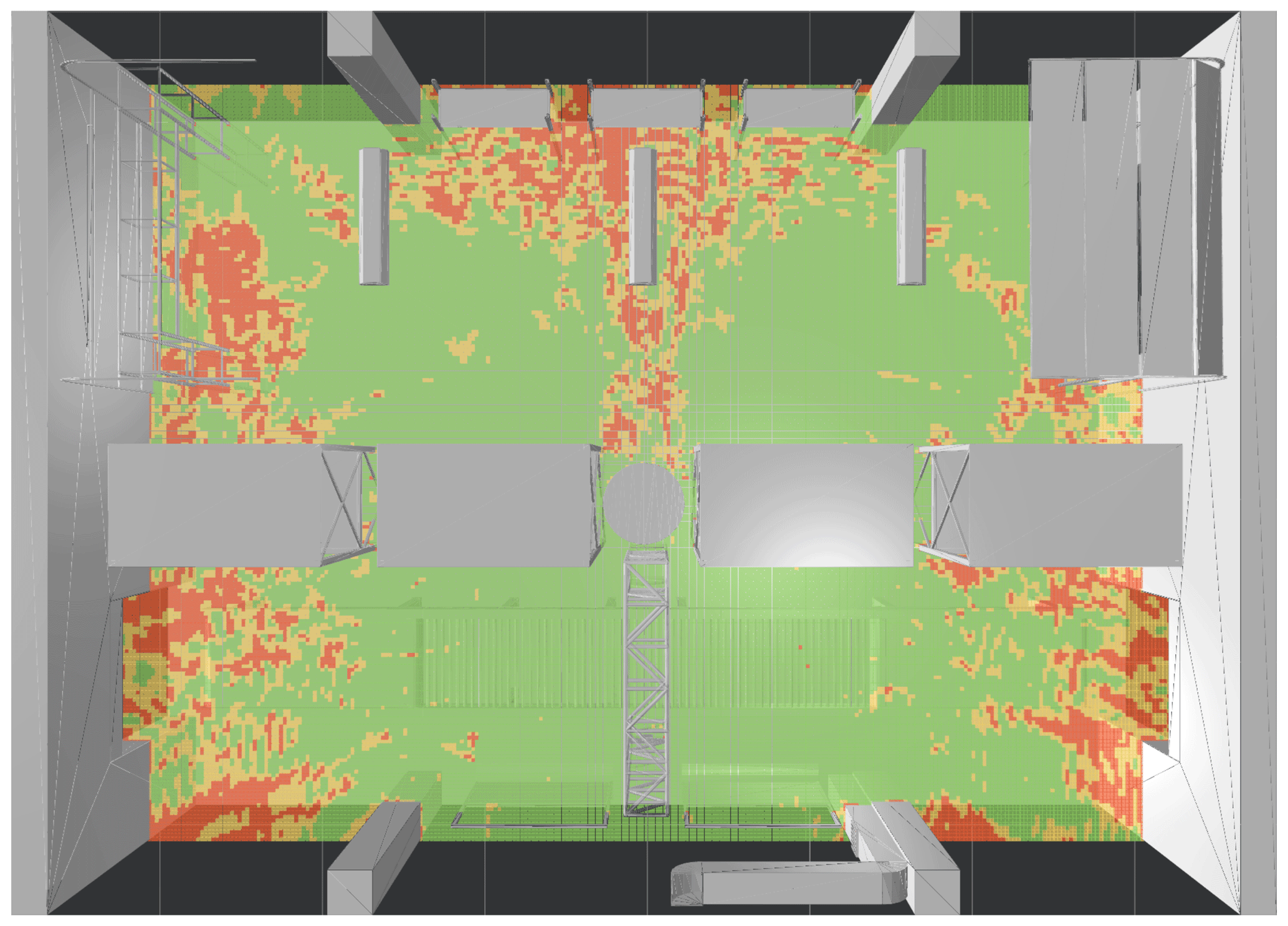
Figure 6 Stage I rating (gate A): Tag locations are classified into three categories: Green locations receive sufficient power, yellow areas mark potentially unreliable spots, red areas cannot be read.

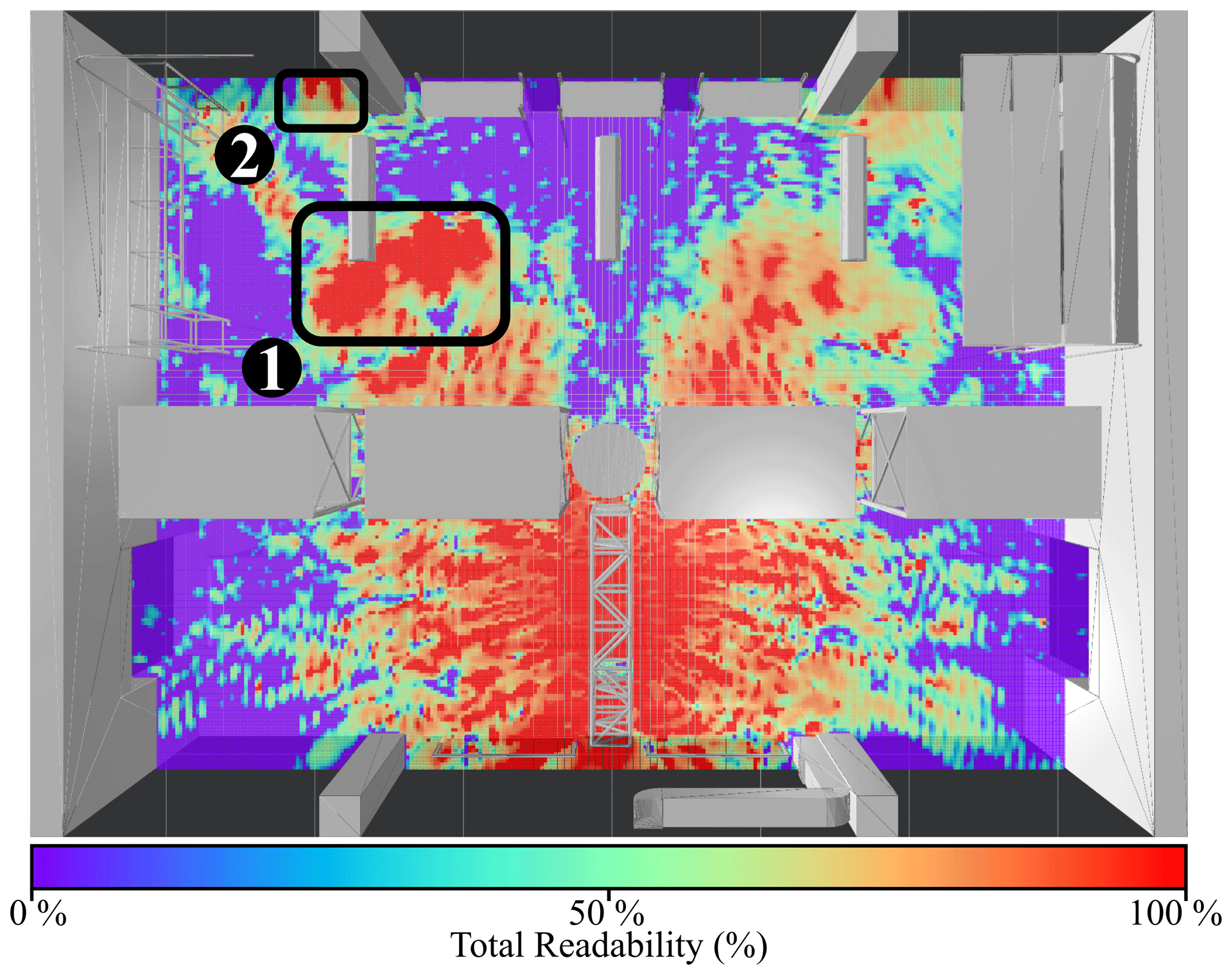
Figure 7 Stage II rating (gate A): Total tag readability R_tag in percent. Two critical spots causing strong overreach are marked with (1) and (2) respectively.

Figure 8 Stage I rating (gate A): Scenario with reduced reader power.

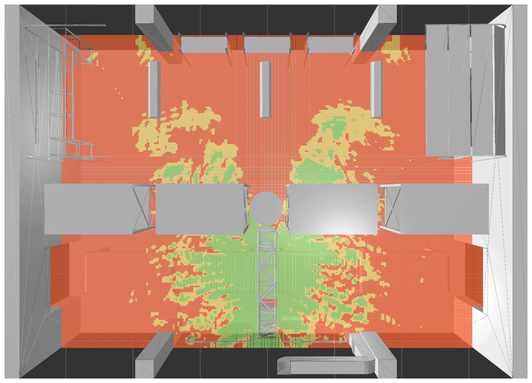
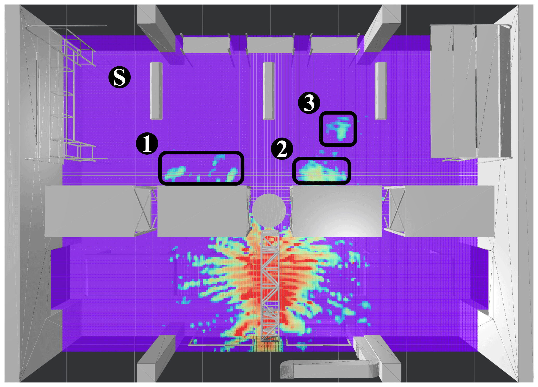
Figure 9 Stage II rating (gate A): Scenario with reduced reader power. Potentially critical spots requiring further investigation are marked with (1), (2) and (3) respectively. Spectator position for the investigation in the 3D environment is marked with (S).

3.2 Analysis of UHF-RFID use-case

This section performs the evaluation of the RFID use-case depicted in Fig. 2, based on the methods proposed in the previous section. Unless otherwise stated, the analysis is performed for a tag sensitivity of $P_{\mathrm{sens}}=-\mathrm{16}$ dBm and an uncertainty factor of ΔF_sens=1. A typical value for antenna gain for a half-wave dipole is G=1.6. However, for the subsequent analysis a gain value of G=1.25 is applied to consider an application specific gain penalty.

The first scenario to be evaluated is the reader antenna at gate A, initially set to emit 2 W EIRP. Figure 6 shows the result of stage I rating in bird's eye view at the height of the gate antenna. The tag reliability is assigned according to the classes defined in Table 2. Tag locations that receive enough power to respond, considering the best case of the computed polarization, are marked with green color. Positions that yield threshold level power and areas with an insufficient power level are colored in orange and red respectively. Figure 7 displays the results of stage II rating, with the color scheme applied for the rating depicted below. As previously explained, tag readability ranges between 0 % and 100 %, depending on how many polarization states yield enough power. As expected in a highly reflective multipath environment, strong interference effects are present. Overall, it is obvious that the applied reader power of 2 W EIRP is way too high for the intended application. Again, reminding of Fig. 2, the storage room area (upper half of the hall) should not be covered by the reader at gate A. Gate A should scan goods transported by the conveyer belt only. Goods present in the storage room should solely be managed by gate B and gate C, keeping track of the current stocking. Two areas exhibit an especially strong overreach, marked with (1) and (2) in Fig. 7 respectively. To draw a conclusion, the emitted reader power must be reduced.

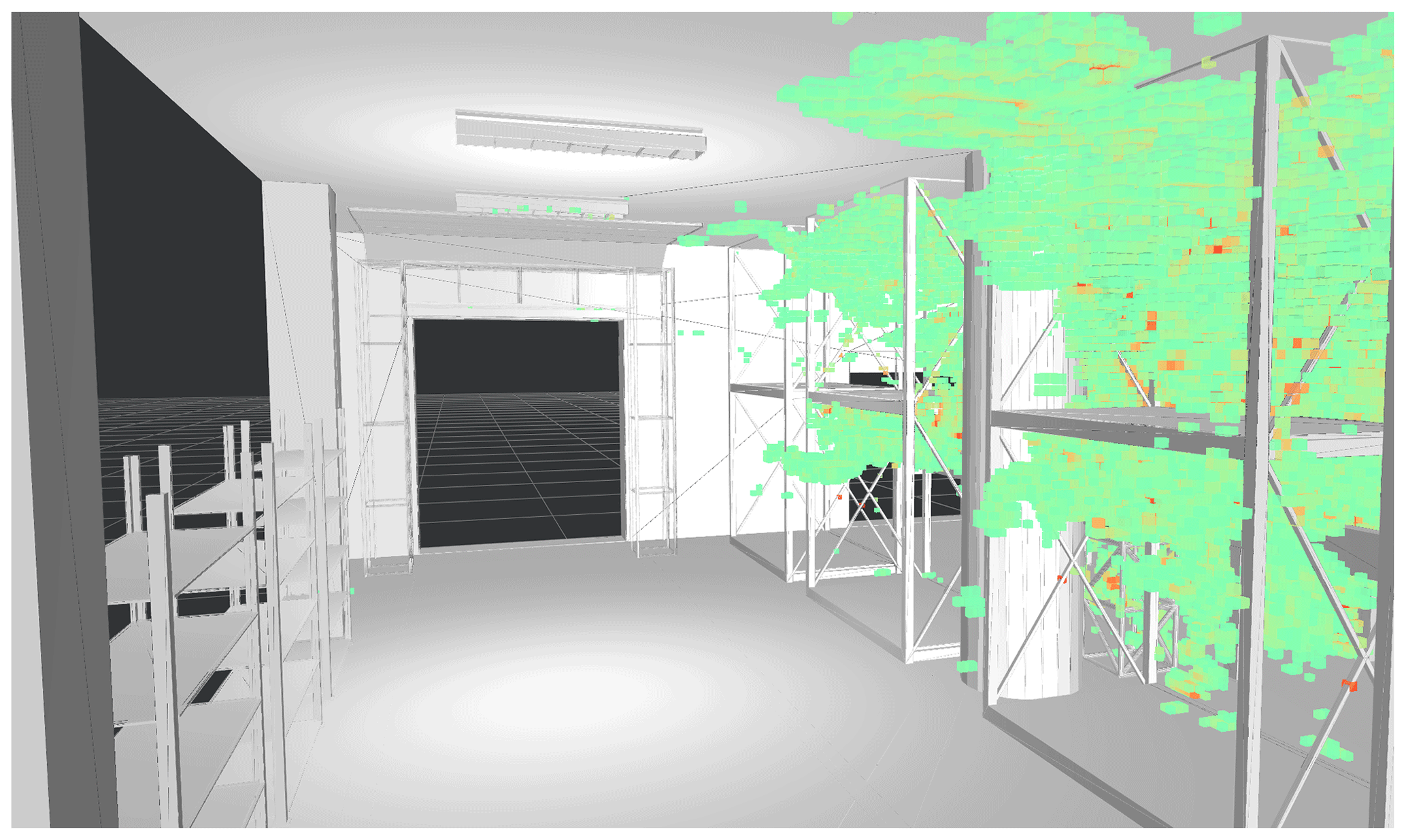
Figure 10 Stage II rating (gate A): Tag locations rated with a readability of at least 50 % analyzed in a 3D environment.

The evaluation is repeated for the same scenario with reader power adjusted to 0.25 W EIRP. Figures 8 and 9 show stage I and stage II rating results for the lowered reader power scenario. Evidently, the operational range has been decreased significantly. However, some smaller overreach spots with significant readability still persist (30 %–60 % of states can be read) and require further investigation. Those areas are marked in Fig. 9 with (1), (2) and (3) respectively.

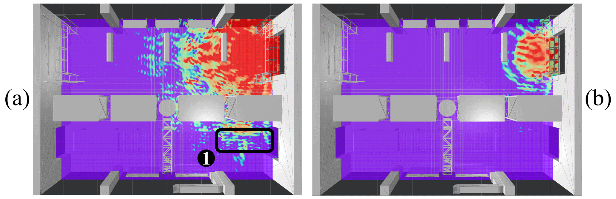
Figure 11 Stage II rating (gate B): (a) An undesired overreach area, which includes the conveyer belt, is present (1). Decreasing the reader power eliminates the critical spot (b).

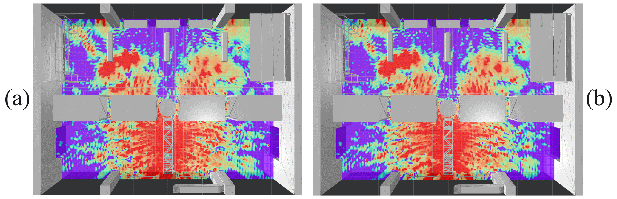
Figure 12 Stage II rating (gate A): Rating results based on FIT (a) and MoM (b) simulation respectively. Good agreement can be verified.

It is very powerful to investigate critical areas in a 3D environment. Figure 10 shows a 3D view from the spectator position marked with (S) in Fig. 9. The applied color scheme is the same as for the 2D readability evaluation and can be recalled in Fig. 7. While the remaining overreach areas could possibly be resolved by further reducing the reader power, another issue becomes obvious in Fig. 10. With the intention of storing goods in the racks (that should not be in reach of the reader at gate A), the logistical conception analyzed in this scenario is problematic. As the logistics environment is still in planning phase, this information can be fed back into the planning process in an iterative manner to deduce possible solutions with important optimizations. For example, the racks could be moved to the other side of the hall, the reader at the gate could be attached facing the other direction, or adequate obstacles could be installed to shield the storage room.

The same evaluation is performed for the reader at gate B. Figure 11 shows an undesired overreach area (marked 1), including a part of the conveyer belt (a). Also, care must be taken in case the dock door is used for direct unloading of goods from trucks. The high power leaving the depot through the dock door in panel (a), could lead to unintended reads during truck unloading. To avoid unintended reads, the power again is decreased to 0.25 W EIRP, eliminating the critical spot (b).

3.3 Validation of simulation results

Convergence studies are not feasible for large-scale simulations due to their time and memory requirements. Performing measurements is not an option either, as the environment is still in its planning phase. Thus, another method is required to confirm the validity of the simulation results. One possibility is the cross-validation of simulation results from two fundamentally different simulation techniques. Under the assumption that the underlying physics are modelled correctly, the solution of both simulation techniques should agree (, ), if the discretization took the geometric structure, its material properties and the phase information of the propagating wave into account correctly. Therefore, a qualitative comparison for the evaluated scenario is made, including results from the FIT and MoM simulation technique.

Figure 12 compares the computed readability rating for the first case evaluated (gate A radiating 2 W EIRP) based on the FIT (a) and MoM (b) simulation respectively. Despite some minor differences, the results of both simulations clearly match to a high degree. Major spots of overreach, as well as interference patterns can be found agreeing in both simulations.

4 Conclusions

Deterministic simulation approaches have been utilized to analyze the signal coverage and interference effects in UHF-RFID-systems. A logistical use-case has been set up and analyzed, based on results obtained from popular full-wave methods. Necessary steps to set up numerical large-scale simulations such as the introduction of equivalent source representations and adequate meshing techniques have been discussed. To facilitate the interpretation of simulation results, a two-stage process for tag readability rating has been proposed and demonstrated on the presented use-case. Critical flaws in the planned system could be identified and adequate countermeasures have been deduced. Finally, a cross-validation of the simulation results has been conducted, confirming the validity of the performed simulations.

Performing accurate a priori readability evaluation utilizing full-wave techniques in combination with adequate rating and visualization methods is a powerful way to uncover flaws in planned systems. As a result, expensive and time-consuming subsequent modifications of the RFID-system and its operational environment can be avoided. This insight might not only lead to a financial benefit for the single operator, but in the long run also increase the trust of yet doubtful enterprises to dare the transition towards RFID technology.