3D Contour Shaping of Buried Objects in Soil

The basic question of this paper was, whether a detected anomaly found in the ground during an explosives disposal process is actually a non-detonated bomb or non-dangerous metallic scrap. Based on a borehole radar, an approach is to be presented in which first a 2-dimensional contour of the object is created with the aid of a spatial runtime evaluation. By repeating this step at different depths with subsequent graphic overlay, a 3D shape of the buried object is created. The method is first tested using a simulation model with inhomogeneous soil. In the second step the method will be applied and evaluated using a field measurement of a real object. The results shows that both 2D and 3D evaluations reflect the position and orientation of the object. Furthermore, the shape and the dimensions can be estimated, with the restriction that the 3D contour has distortions along the vertical axis. The aim of this work is to show an application of borehole radar, with which the identification of buried objects should be facilitated.

1 Introduction

As a result of the First and Second World War, an enormous amount of 2.7 million t of bombs and other explosive devices were dropped over Europe. Some of these are still a major threat today, as estimated 10 % did not detonate on impact and are thus hidden in the ground as so-called buried unexploded ordnances (UXO). The construction industry is particularly at risk, as these objects can be located up to a depth of 10 m. In order to counteract this danger, institutions were created in many countries to locate, recover and to dispose of these UXO, such as the explosive ordnance disposal (EOD) service in Germany.

There are many methods for the detection of buried objects which are based on different physical effects and can be further subdivided into surface methods and borehole methods. The most common methods are magnetic methods in which the earth's magnetic field is evaluated and searched for distortions caused by magnetic objects, electromagnetic methods in which the conductivity of metallic objects is used to stimulate eddy currents and the ground penetration radar in which short electromagnetic pulses are emitted and the echoes are evaluated. All these methods have in common that, depending on the soil properties, it is possible to detect a buried object relatively reliably. In addition to the position, an approximate volume of the object can be determined as well. However, identification often proves to be difficult and thus occasionally leads to the excavation of non-hazardous metallic scrap. In order to carry out a more precise classification, an electromagnetic “fingerprint” is created from the recorded measurement data (Won et al., 2001). This is then compared with existing databases of known objects, taking into account the determined volume (Billings, 2004). However, if the buried object is not represented in the database, identification remains challenging.

This work deals with an application of the Borehole Ground Penetration Radar (BHGPR). The special feature of this method is that several Boreholes are created around the presumed position of the hidden object. Thus, information about the object can be obtained from a variety of directions and angles. This data will be used to carry out a graphical reconstruction of the object shape and thus represent an identification method without the aid of databases. Theoretical considerations and a 2D reconstruction with the help of simulations have already been presented in Siebauer et al. (2019). In this work, the approach is expanded to include a 3-dimensional evaluation and verify it with the help of measurement data in addition to simulations. The method requires that the position of the object to be examined has been approximately determined beforehand. It is particularly expedient to also use the BHGPR as the initial detection method, since those measurements can be re-used with the approach we present here.

2 Simulation setup

The aim of the simulation setup is to reproduce the setup of a real BHGPR measurement. The boreholes required for this are drilled in a predefined grid around the suspected point at a depth of several meters. Figure 1 shows the arrangement of the drill holes in the simulation model and the positioning of the hidden object (DUT). The boreholes are arranged in rows with a distance of 1.5 m between each row and within the row by 1.5 m. The open source software gprMax (Warren et al., 2016) is used for the simulation. This was specially developed for simulating Ground Penetrating Radars and uses the FTDT method. In addition to homogeneous soil, it is able to reproduce more complex inhomogeneous soils.

Figure 1 Borehole pattern of simulation with DUT.

2.1 Simulation space

The simulation space comprises 8 m × 8 m in the horizontal plane (x and y direction) and 3.2 m in the depth which was discretized in 1.2 cm × 1.2 cm × 1.2 cm cubes. The upper 20 cm of the space consist of vacuum to be able to simulate ground-air reflections. For the modeling of the remaining 3 m a mixing model for soil by Peplinski et al. (1995) was used, which is implemented directly in gprMax. The Peplinski soil was mixed with the help of a fractal distribution in such a way that the inhomogeneities occur more in the z-direction and vary less strongly in the horizontal plane. A vertical section through the simulation room is given in Fig. 2 and is intended to give an idea of the soil model. The material properties vary for the relative permittivity between ε_r=4.0–5.6 and for the conductivity between σ=0.019–0.038 S m⁻¹.

Figure 2 Section through simulation model.

For the excitation of the GPR signal, a Hertzian dipole antenna with z-alignment is used, which is moved along the borehole depth for all hole positions. The echo signal is evaluated using a field probe, which is positioned 10 cm below the antenna. A Ricker wavelet (mexican hat wavelet) with a center frequency of 400 MHz is used as the feed signal. The selected frequency range plays a major role in GPR, as frequencies that are too high are attenuated too much by the soil and too low frequencies hardly generate echoes on the small DUTs. Another important parameter is the signal bandwidth, since an increase leads to a shorter pulse in the time domain, which improves the spatial resolution. The Ricker pulse used in the simulation has a −10 dB bandwidth of 588 MHz or a −3 dB bandwidth of 329 MHz in the power spectrum.

2.2 Hidden object

The hidden object which was used for the simulation, see Fig. 3, was modeled after the 100 pound bomb AN-M 30 without tail unit, as this is a common hazardous object in the EOD service and is at the lower end of the detectable size with a BHGPR. It has a length of 76 cm, a diameter of the main section of 21 cm and is modeled as PEC. Starting from the center of the borehole grid, the object was shifted 0.5 m in negative x and y​​​​​​​ directions and placed at a depth of 1.5 m. The alignment of the body is parallel to the x-axis.

Figure 3 Simulated hidden object in gprMax.

3 Methodology

3.1 Determination of soil properties

The first step is to determine the soil properties. As a simplification, it is assumed that the soil properties remain approximately constant along a layer depth. For this purpose, reference measurements in the form of transmission measurements are carried out in at least two boreholes. Holes that are not in the immediate vicinity of the DUT are suitable here, as the DUT echoes could interfere with the measurement. In the simulation, the DUT was removed from the ground for this purpose. The transmitting antenna and the field probe are held at the same height. They are then moved along the depth of the borehole and the signal transit time t_t(z) is measured for each depth. In addition to the runtime, the delay time t_d of the measuring system is required and can be determined by a reference measurement in air with a known antenna distance. With Eq. (1) and the constant c₀ for the speed of light in a vacuum, the relative permittivity of the soil a long the depth z can be calculated.

$$\begin{array}{}\text{(1)}& {\mathit{\epsilon }}_{\mathrm{r}}\left(z\right)={\left({\displaystyle \frac{t_{\mathrm{t}}\left(z\right)-t_{\mathrm{d}}}{c_{\mathrm{0}}}}\right)}^{\mathrm{2}}\end{array}$$

3.2 Evaluation of the echo data

Before the echo data are evaluated in the next step, it is usually necessary to carry out post-processing on the raw data. This helps with interpreting the data and can make weak echoes visible. When plotting the echo data from a borehole measurement, the echoes from the DUT become apparent as hyperbolas. These are manually picked inside Matlab for each borehole and it is stored at which time t_r(z) the echo occurred for each depth. An example from the simulation data is shown in Fig. 4 with the DUT's picked echo hyperbola (dashed line). The determination of the DUT position with aid of the previous detection method is of great help, since desired DUT hyperbola can be better separated from undesired clutter echo signals.

Figure 4 Echo hyperbola of the borehole simulation.

3.3 Contour shaping method

This section describes the contour shaping method. Since the assumption is made that each layer height of the soil has a constant speed of propagation, all layer depths are evaluated separately. The time at which the DUT echo to be examined reaches the field probe depends on the distance between the antenna and the closest DUT surface piece and on the propagation speed in the medium. With the help of the previously obtained relative permittivity ε_r(z) of the soil layers, each depth can be assigned a speed of propagation v(z). Since the GPR signal has to propagate twice the distance in order to be received, the antenna DUT spacing is calculated with Eq. (2).

$$\begin{array}{}\text{(2)}& r\left(z\right)={\displaystyle \frac{c_{\mathrm{0}}\cdot t_{\mathrm{r}}\left(z\right)}{\mathrm{2}\sqrt{{\mathit{\epsilon }}_{\mathrm{r}}\left(z\right)}}}\end{array}$$

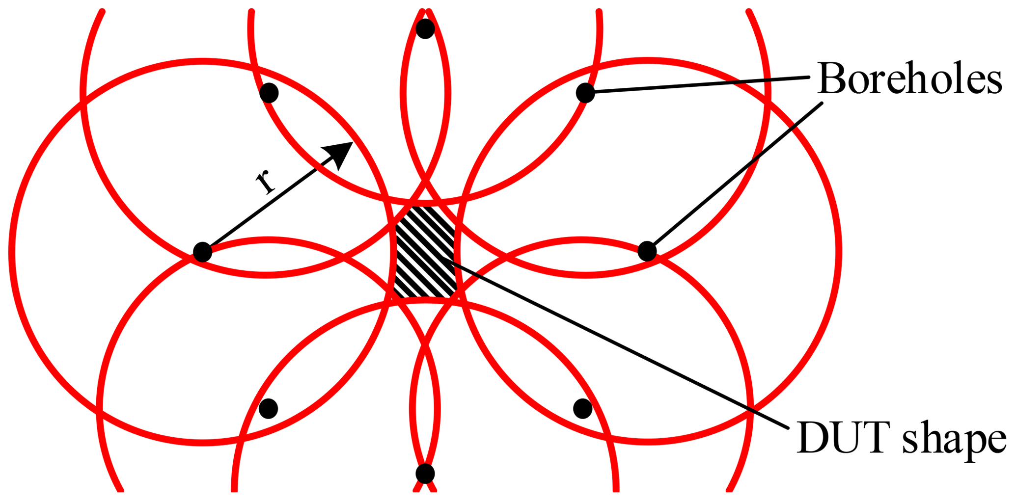
Starting from the respective antenna position, a circle is drawn for each borehole with the determined DUT distance r. If all the circles are superimposed on one another, an area should remain free at the previously determined DUT position. This represents the determined contour of the current borehole depth. Boreholes which do not have a useful DUT echo, for example due to a large distance or due to strong soil damping, are omitted. Figure 5 shows a simplified arrangement with boreholes located on a circular path around the DUT.

Figure 5 2D reconstruction through echo superposition.

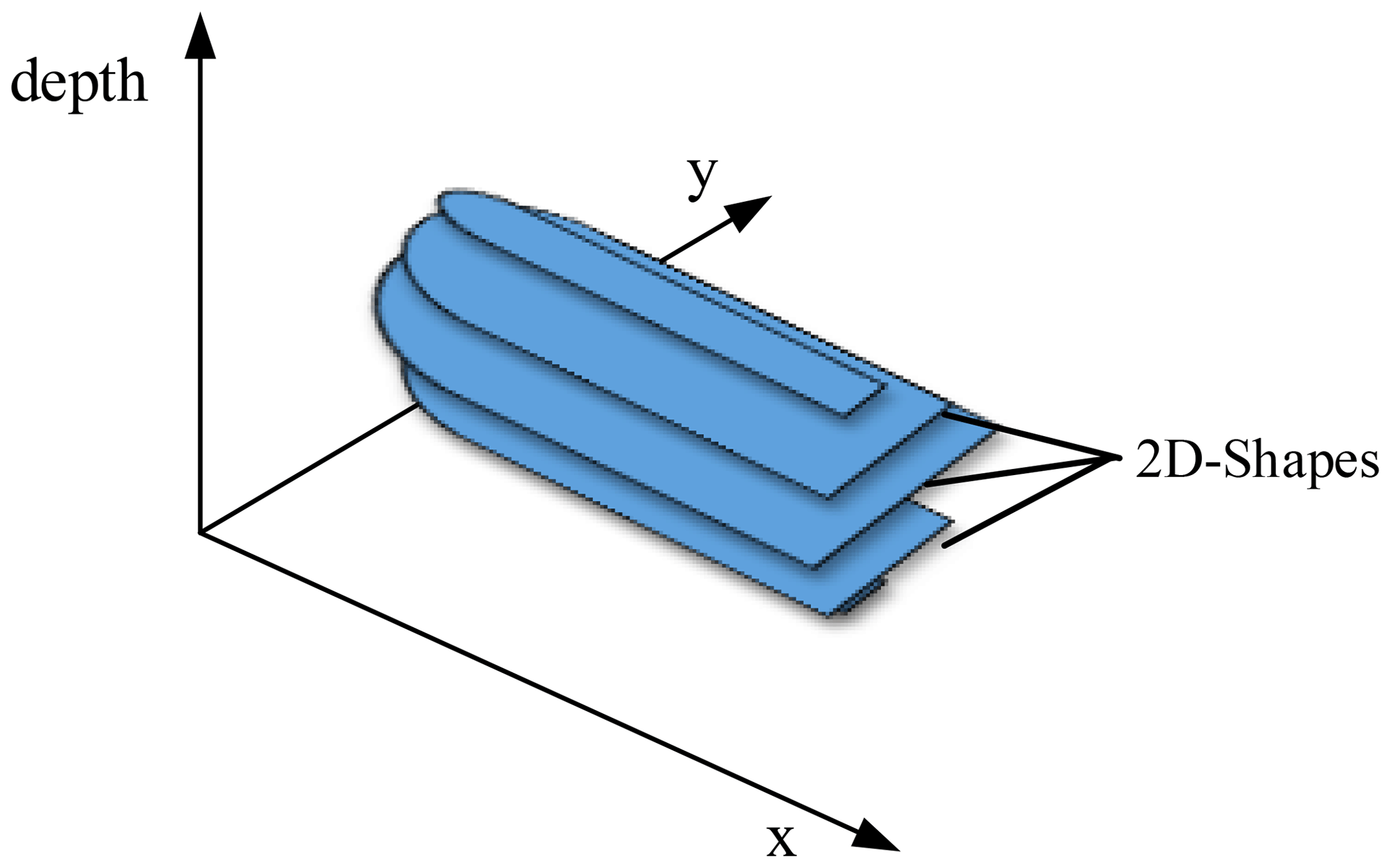
This 2D method is carried out automatically for all layer heights along the borehole depth and then stored in a 3D Matrix. In Matlab, the shapes are graphically overlaid for each recorded depth. Since the free areas of the individual 2D shapes should decrease with increasingly different drill hole depths, a 3-dimensional volume is created at the DUT position. Such an overlay and thus the 3D reconstruction of the object shape is carried out as an example in Fig. 6.

Figure 6 3D reconstruction via shape superposition.

4 Results and discussion

In the following, the reconstruction method will first be applied to simulation data and then to field data. Matlab is used to evaluate the data.

4.1 Evaluation of the simulation model

The following simulation data were generated with the previously presented gprMax model. To make the manual selection of the echo hyperbolas easier, a gain filter and a Dewow filter (Szymczyk and Szymczyk, 2013) were applied to the obtained simulation raw data.

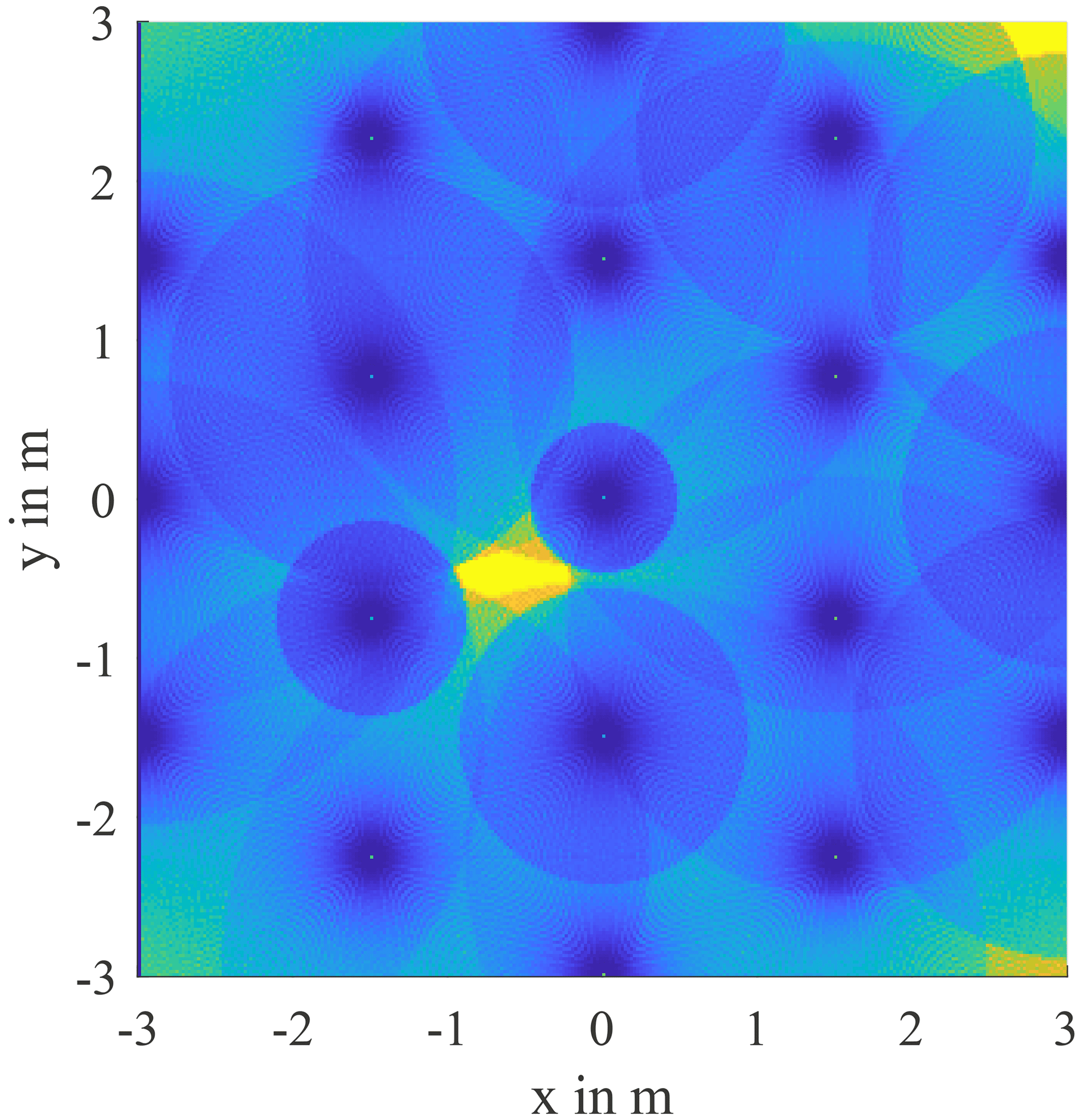
Figure 7 shows the 2-dimensional horizontal section at the level of the DUT. The extend in the x-direction with approximately 74 cm and the extend in the y-direction with and approximately 24 cm, fit well with the DUTs length of 76 cm and diameter of 21 cm. The positioning and alignment also agrees with the expected value. Of the 19 hole positions 14 led to useful overlays. Only the most distant boreholes did not provide any useful hyperbola. Despite the inhomogeneity, this is due to the lack of clutter in the simulated soil.

Figure 7 2D contour (yellow area) of the simulation DUT.

In the next step, the 2D method is carried out automatically for all layer heights along the borehole depth and a 3-dimensional image is created. It should be noted, however, that the more the considered height differs from the actual DUT height, the 2D results have to be treated with caution. This is because the propagation lobe of the transmitting antenna not only radiates along the horizontal plane but also at an angle into the room. As a result, these oblique reflections distort the object vertically (z-direction) in the 3-dimensional representation.

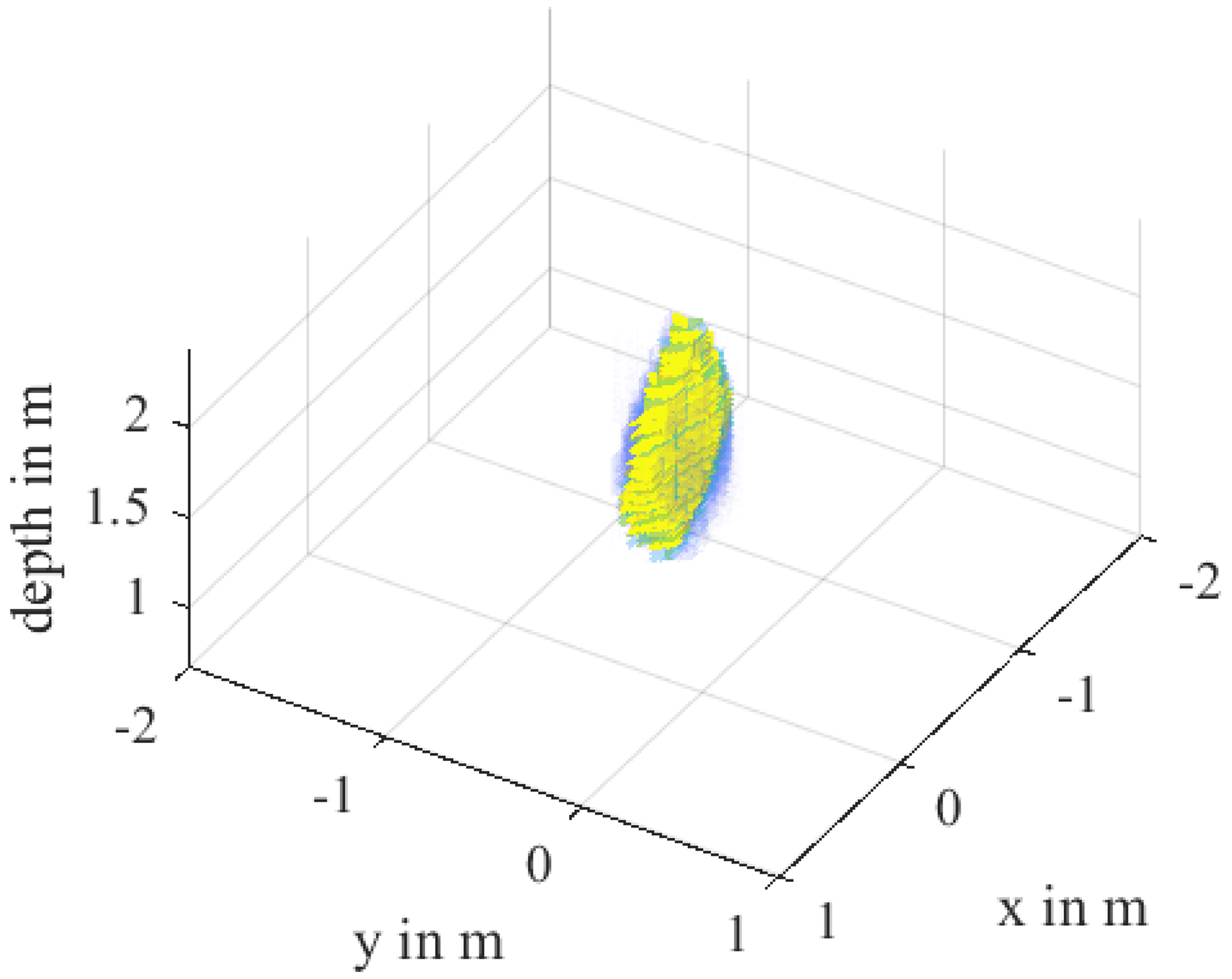
This effect becomes clear in Fig. 8, where the 3D surface reconstruction of the simulation data is shown. The cylindrical body of the DUT is distorted into a circular disk and a z-dimension of 1 m can be measured in the middle. This effect must be kept in mind for the identification of the object or an equalization filter must be developed to compensate this. One possible approach would be to distort the echo hyperbola according to the distance between antenna and DUT.

Figure 8 3D reconstruction of the simulated DUT.

4.2 Evaluation of field data

In the following, the presented algorithm was tested on a real structure on a test site with an existing borehole grid. A defused 500 pound bomb without tail unit was used as DUT, which is buried in sandy soil at a depth of 4 m. Its length is 1.18 m and has a diameter of 36 cm and its shape matches roughly to the model from Fig. 3. The existing borehole grid, which has been created around the DUT, analogous to the one in Fig. 1, has a drilling depth of approximately 6 m. For the reflection measurement, a borehole ground penetration radar system from IDS was used in which the transmitting and receiving antenna are built together into a plastic tube with about 1.2 m length. This system operates with an electromagnetic pulse with a center frequency of 300 MHz and was configured so that a measurement was carried out in 1.1 cm steps along the depth. A second, identical antenna system was used for the transmission measurement to determine the soil properties.

The reference measurements were made on two boreholes secluded from the DUT. The transmitting system and the receiving system were lowered in 1 m steps and a reference measurement was carried out for the respective depths. The values obtained for the relative permittivity ε_r(z), which were in the range ε_r=3.7–5.5, were linearly interpolated in the intermediate ranges.

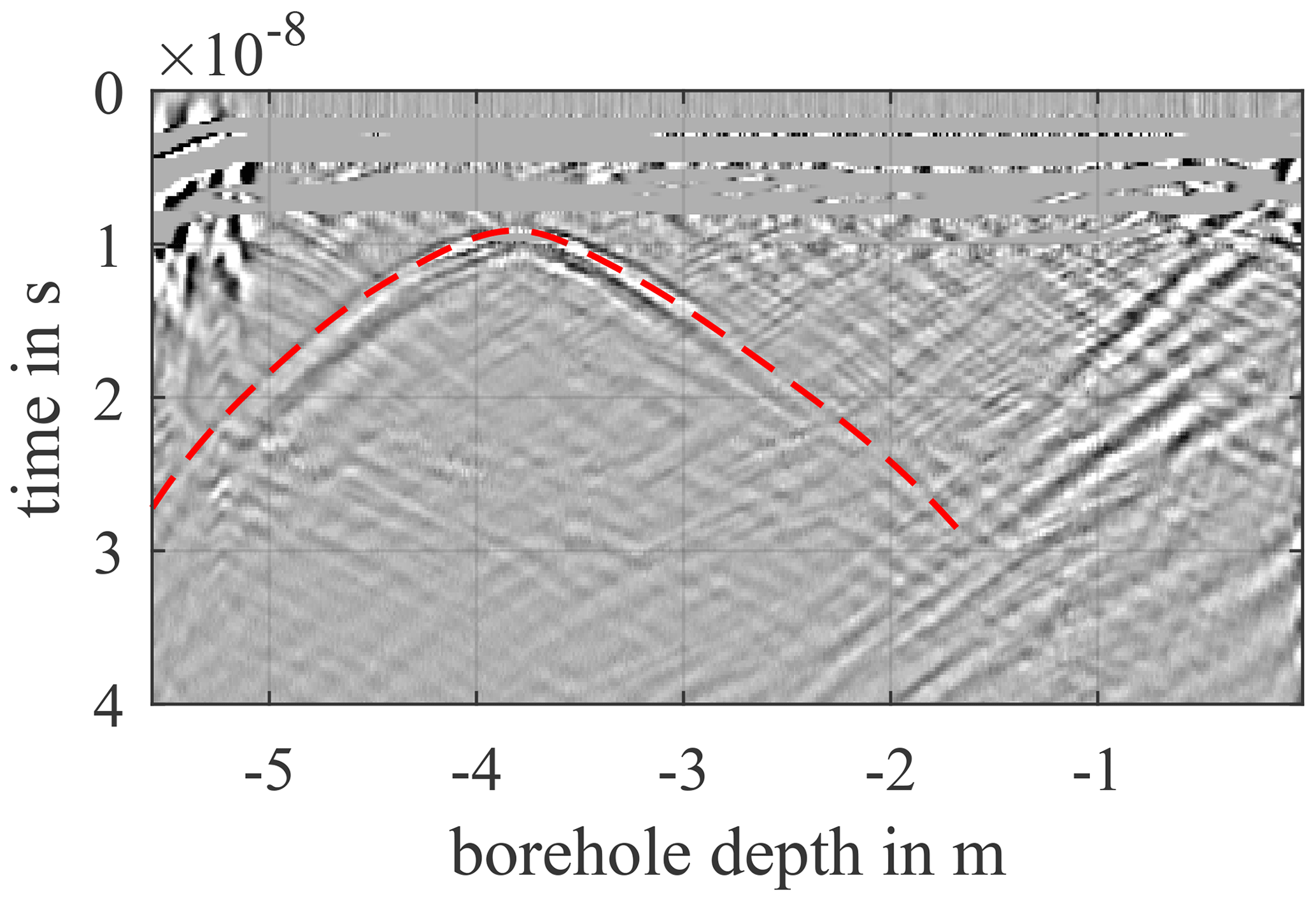
For detecting the echo hyperbolas, the measurement data must be prepared using post processing filter. These are then picked manually in Matlab, see Fig. 9, whereby knowledge of the location of the DUT is also very helpful to distinguish the DUT echoes from clutter. Measurements that do not show a suitable hyperbola or where the result is not clear were deliberately given a short echo time. As a result, these measuring points have no disruptive effect in the subsequent reconstruction.

Figure 9 Echo hyperbola of the filtered measurement data.

First, the 2-dimensional reconstruction at DUT height, which is shown in Fig. 10, should be examined. Relatively in the center of the drill hole grid, a free space can be seen, which represents the determined contour of the DUT. Of the total of 19 drill holes, only 7 led to useful overlaps. The actually expected cylindrical shape shows a “bulge” on the right side (in the direction of the positive x-axis). The reason for this is that the measurement marked with a red ring does not have a characteristic hyperbola and therefore the outer contour is not correctly reproduced from this direction. If one takes this into account, a lot can still be deduced from the measurement.

Figure 10 2D reconstruction of the field measurement.

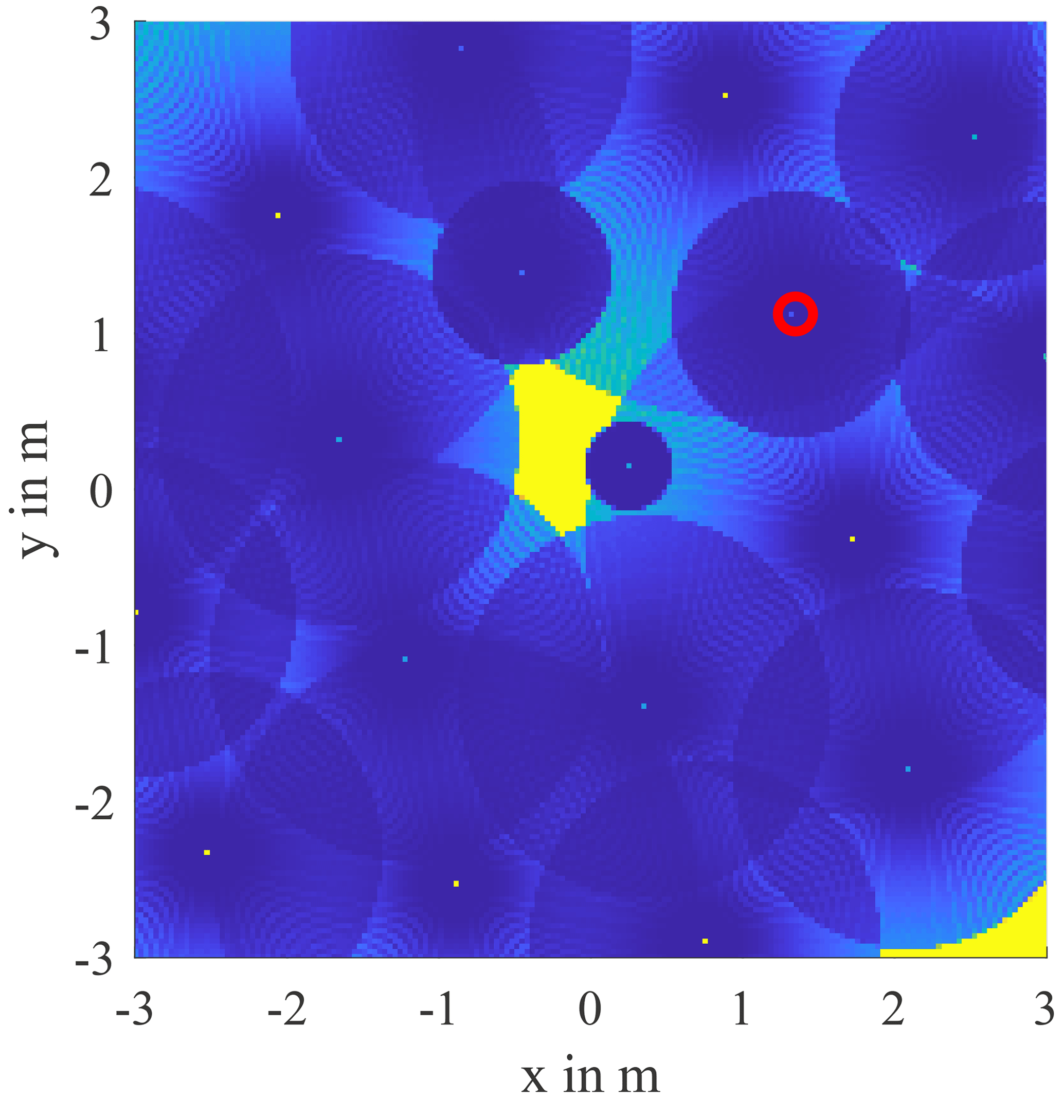
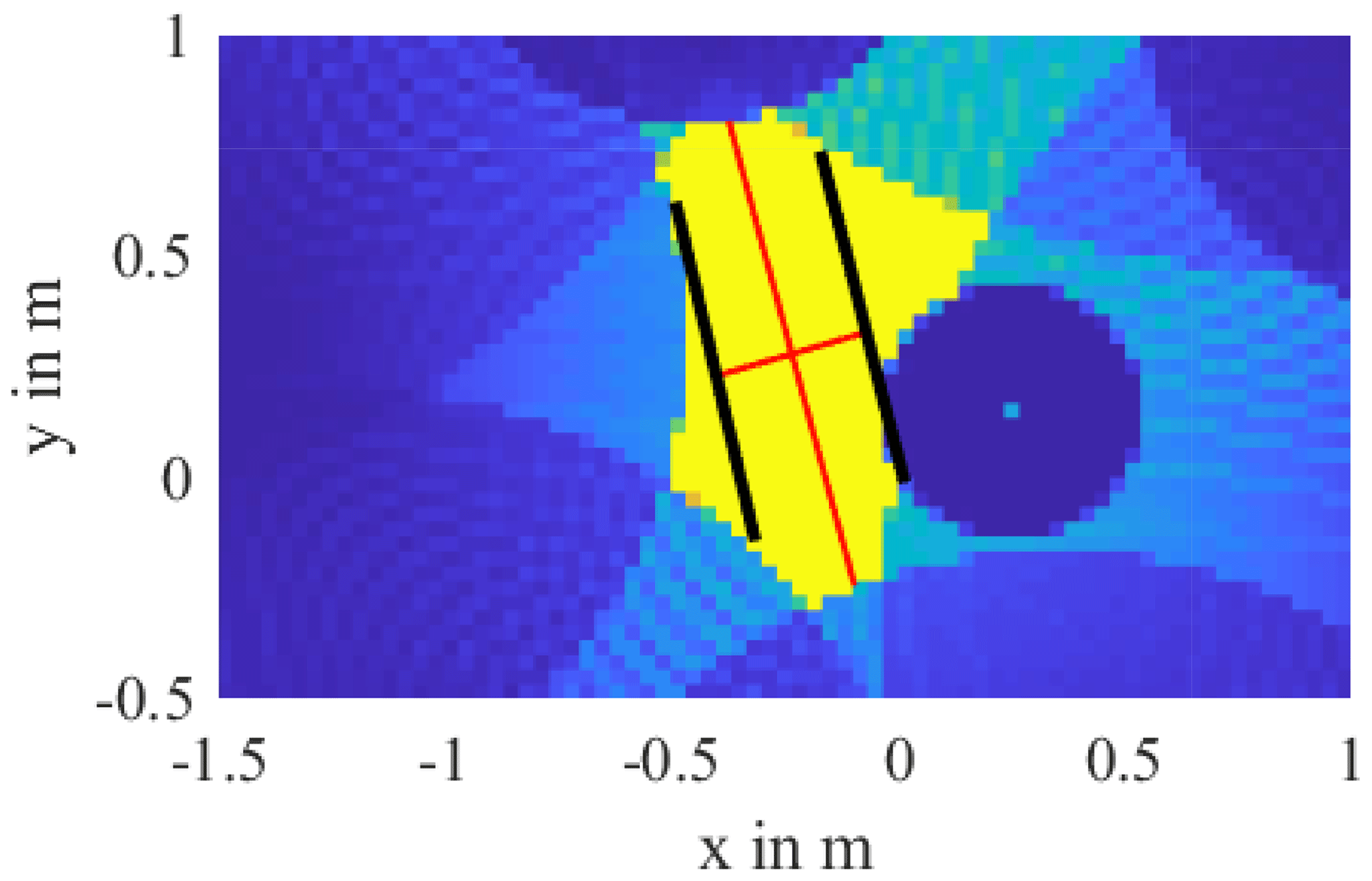
Figure 11 shows a close-up of the DUT area. Here the length and width of the body, represented by red lines, were read off. The determined length is 1.10 m and thus roughly corresponds to the expected 1.18 m. Reading the diameter is a bit trickier. For this purpose, two parallel straight lines were drawn in symmetrically to the estimated DUT alignment so that they touch the trustworthy echoes. The width determined in this way is 35 cm and therefore corresponds very well to the expected DUT diameter of 36 cm. The accuracy of the determined contour depends on several factors, in particular on the homogeneity of the soil and how exactly the propagation speed of the medium was determined. In addition, the best 2D results are obtained when the evaluation is carried out at the depth of the DUT, since here the effects of the z-axis distortion do not occur or occur to a minimum.

Figure 11 Determination of the object dimensions.

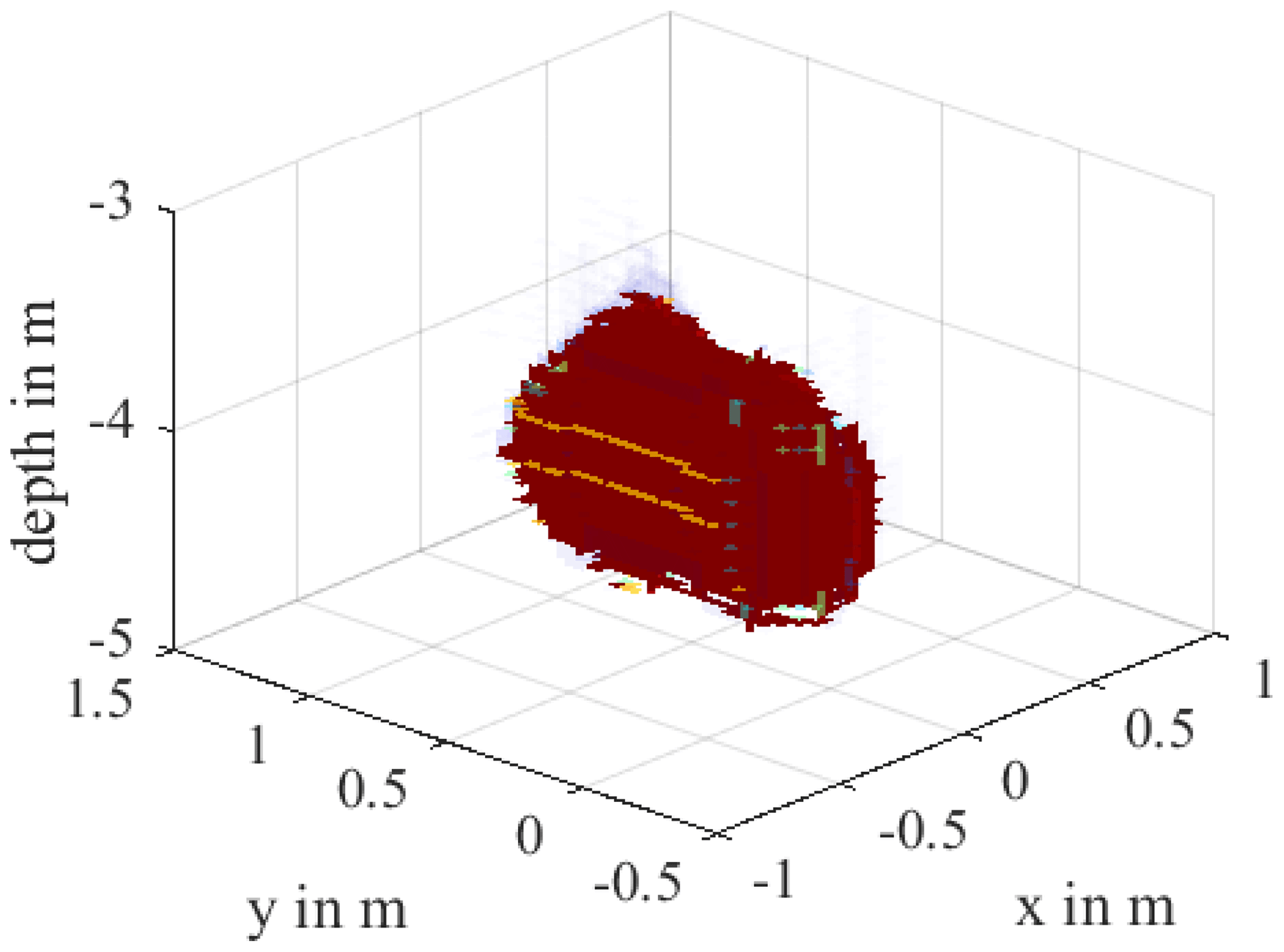
The result of the 3D evaluation is shown in Fig. 12. A geometry can be recognized which resembles a capsule. Here you can see that the reconstructed geometry, like the real DUT, is aligned flat in the ground at a depth of 4 m. As with the reconstruction of the simulation data, the body is stretched along the z-axis. The measured maximum z-extension of the body is 1.3 m.

Figure 12 3D reconstruction of the field measurement.

Because 6 of the 7 boreholes that contributed to the reconstruction were within a radius of 1.7 m, it could be shown that it is not advisable for identification to create boreholes that are far away from the DUT. Instead, if security allows, these should be placed in a smaller radius around the DUT. Despite the relatively low yield of useful boreholes, an object contour could still be reconstructed, with which the dimensions, orientation and general structure of the body could approximately be recognized.

5 Conclusions

The detection and subsequent disposal of non-detonated explosive devices from the times of the First and Second World Wars is a laborious and expensive task. The identification after previous detection of a buried object is a challenge here. This work deals with a contour-shaping method based on borehole ground penetration radar and enables, with the aid of a spatial runtime evaluation, both a 2-dimensional and a 3-D visualization of the buried object. First a simulation model was developed with the help of the open source software gprMax, which simulates a BHGPR measurement in inhomogeneous soil. Here it was shown that the shape and orientation of the object was reproduced well in the 2D reconstruction. The method of 3D contour shaping showed distortions in the z-direction though. A possible solution for this effect would be the development of an equalization filter or an additional measurement by a surface GPR. Nevertheless, position, alignment and general contour could also be estimated here. In the second part of the work, the procedure was applied on a BHGPR test site with a real DUT. It turned out that both 2D and 3D evaluations are possible even with a relatively small number of detected echoes. The dimensions, the orientation in the ground and the rough shape of the body could be reproduced. However, it was also shown that only boreholes with a small distance to the DUT (<1.7 m) contributed to the reconstruction. It can be concluded from this that the method presented can be used to visualize and better identify a detected buried object. For optimal results, a drill hole grid with a small distance to the object is necessary.