 | 21 Feb 2022
Far- and Near Range Measurements with a Synthetic Aperture Radar for Educational Purposes and Comparison of Two Different Signal Processing Algorithms
Jonas Berg
Simon Müller
Andreas R. Diewald
In this paper two simple synthetic aperture radar (SAR) methods are applied on data from a 24 GHz FMCW radar implemented on a linear drive for educational purposes. The data of near and far range measurements are evaluated using two different SAR signal processing algorithms featuring 2D-FFT and frequency back projection (FBP) method (Moreira et al., 2013). A comparison of these two algorithms is performed concerning runtime, image pixel size, azimuth and range resolution. The far range measurements are executed in a range of 60 to 135 m by monitoring cars in a parking lot. The near range measurement from 0 to 5 m are realised in a measuring chamber equipped with absorber foam and nearly ideal targets like corner reflectors. The comparison of 2D-FFT and FBP algorithm shows that both deliver good and similar results for the far range measurements but the runtime of the FBP algorithm is up to 150 times longer as the 2D-FFT runtime. In the near range measurements the FBP algorithm displays a very good azimuth resolution and targets which are very close to each other can be separated easily. In contrast to that the 2D-FFT algorithm has a lower azimuth resolution in the near range, thus targets which are very close to each other, merge together and cannot be separated.
- Article
(9690 KB) - Full-text XML
- BibTeX
- EndNote


The synthetic aperture radar (SAR) is a commonly used imaging radar technique to generate two-dimensional images for the detection and reconstruction of objects or landscapes. The SAR is mainly implemented in aircrafts or satellites to achieve very large ranges and also high angular resolutions (Ulander et al., 2003; Gorham, 2010; Wolff, 2021). The common SARs are used in aerospace to generate high resolution radar images. For educational purposes a 24 GHz (ISM) FMCW radar system was implemented on a linear drive in order to teach students two different radar imaging methods in the university education and to show them the different drawbacks and advantages of these methods. Using various signal and SAR processing algorithms a radar image of a parking lot in the far range was generated from the acquired data. The methods are intuitive and well known. The frequency backprojection method is described in Gorham (2010). Furthermore measurements of several targets in the near range are recorded and processed. The goal is to teach students different algorithm approaches that achieves different angular resolution either in the far or the near range, taking into account the runtimes and variable parameters. In Sect. 2 the operation of the SAR is described shortly and some different recording methods are compared. In Sect. 3 the intuitive 2D-FFT SAR processing algorithm is given and the required equations are shown. Section 4 describes the frequency backprojection (FBP) algorithm with theoretical examples. The comparison of the two methods based on measurements is given in Sect. 5 for the far range and in Sect. 6 for the near range. A final conclusion is given in Sect. 7 which summarizes all results.
The paper itself is comparable to the educational document of the laboratory experiment at the university. Section 1 up to 4 describes the method. Furthermore a instruction of how to acquire the data is given. The results of Sects. 5 and 6 are not shown to the students, these have to been generated by the students in the experiment and should be compared and conluded on there own.
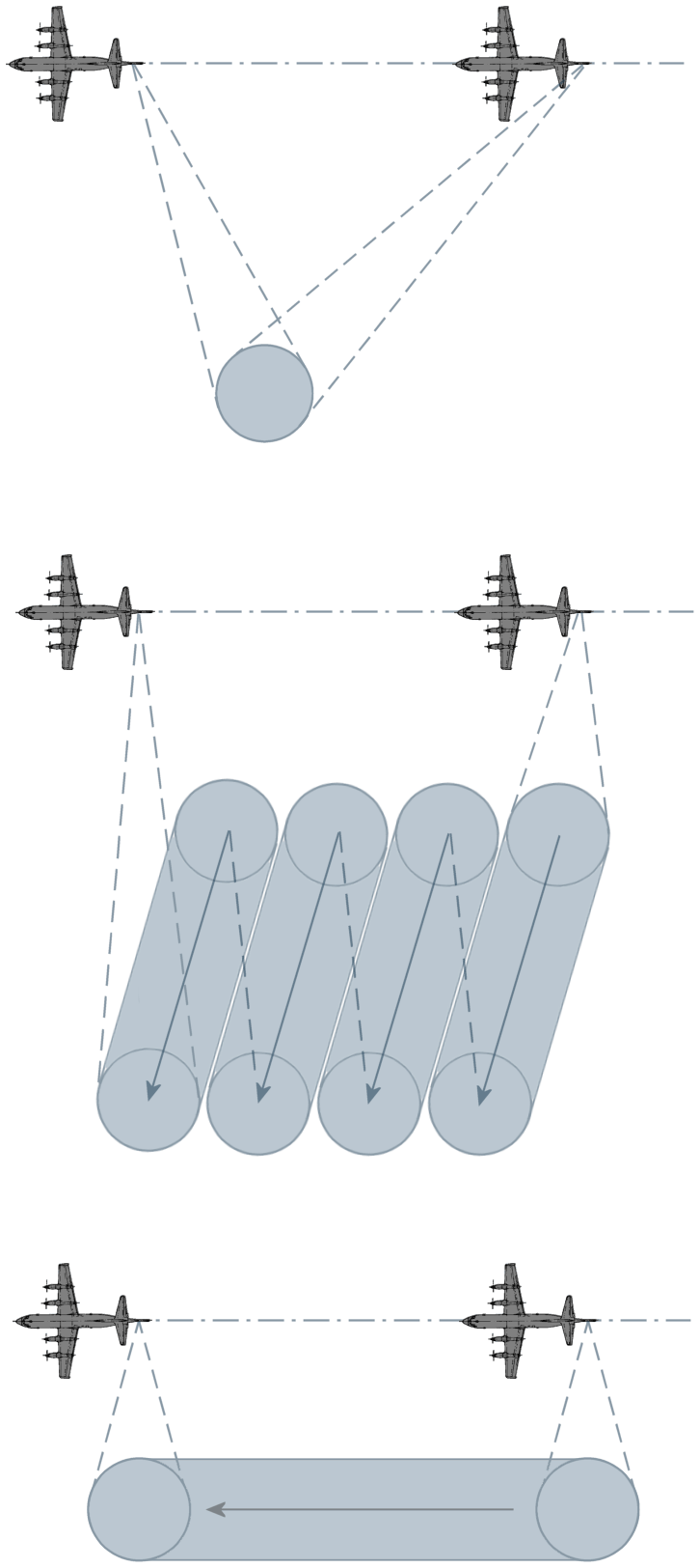
A synthetic aperture radar is commonly used in space and aviation to produce high-resolution radar images of objects or landscapes. The synthetic aperture is an artificial enlargement of the radar antenna to obtain a better azimuthal resolution. This is achieved by mounting a radar system on a moving platform and send out radar signals at constant intervals. The spatial shift of the antenna produces a plurality of imaginary radar antennas similar to a phased array antenna. Depending on the application, this results in several hundred or thousand imaginary antennas, which contribute to a very high angular resolution. There are several SAR procedures like Stripmap-SAR, Spotlight-SAR, and Scan-SAR which are shortly depicted in Fig. 1.
-
Spotlight-SAR: With the spotlight SAR, the antenna is aimed at a specific target area (spot) for a long time which causes the antenna to be rotated in azimuth. This achieves a higher resolution in the spot, but reduces the maximum imageable area (Wolff, 2021).
-
Scan-SAR. The scan SAR can cover several subregions by periodically switching the antenna alignment. This does not have to happen comprehensive. An advantage of the Scan-SAR is that very large areas with multiple target areas can be scanned (Wolff, 2021). The different spots can be in different positions, between which there may be areas that do not need to be detected by the radar.
-
Stripmap-SAR. The stripmap SAR is the standard procedure where the antenna is in a fixed position and directed diagonally towards the surface to be illuminated. The aircraft with the radar system moves on a straight trajectory at a constant speed and emits the radar signals at regular intervals (Wolff, 2021).
2.1 Radar system implemented on a linear drive
Similar to the stripmap-SAR a SAR method was applied for measurements across a moving platform. However, the radar system was mounted on a linear drive and moved stepwise only over a small distance of 2 m. Thus, a straight-line but stepwise movement was generated and the radar signals were sent time-independent.

Figure 2Radar position, © Google Maps 2021 (Google Maps, 2021).
This procedure has made it possible to scan a area of more than 13 000 m2 with a laboratory radar of 100 mW of transmit power and to identify individual objects.
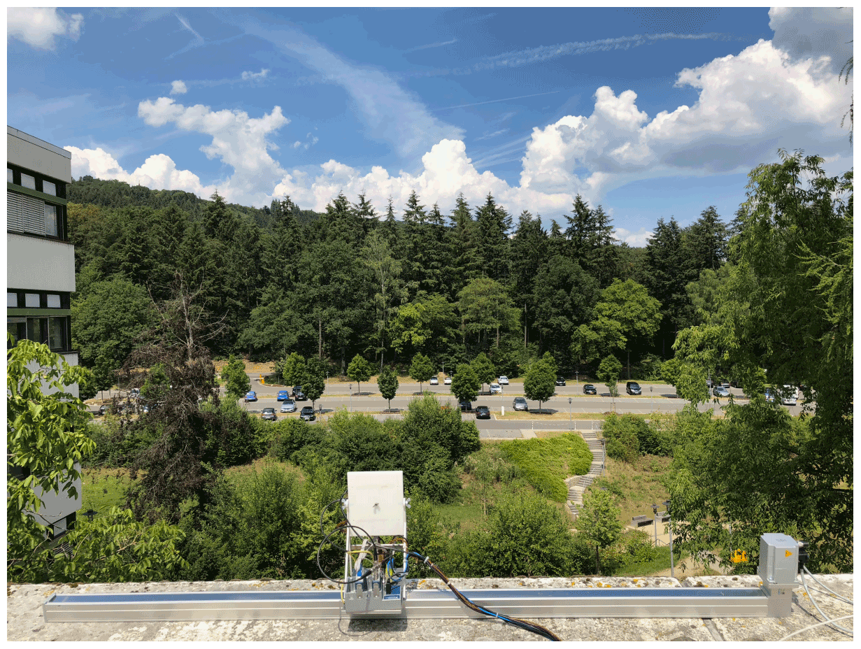
Figure 2 shows the radar measurement location for observation of the university parking lot and and the measurement setup itself in Fig. 3.
2.2 Radar system
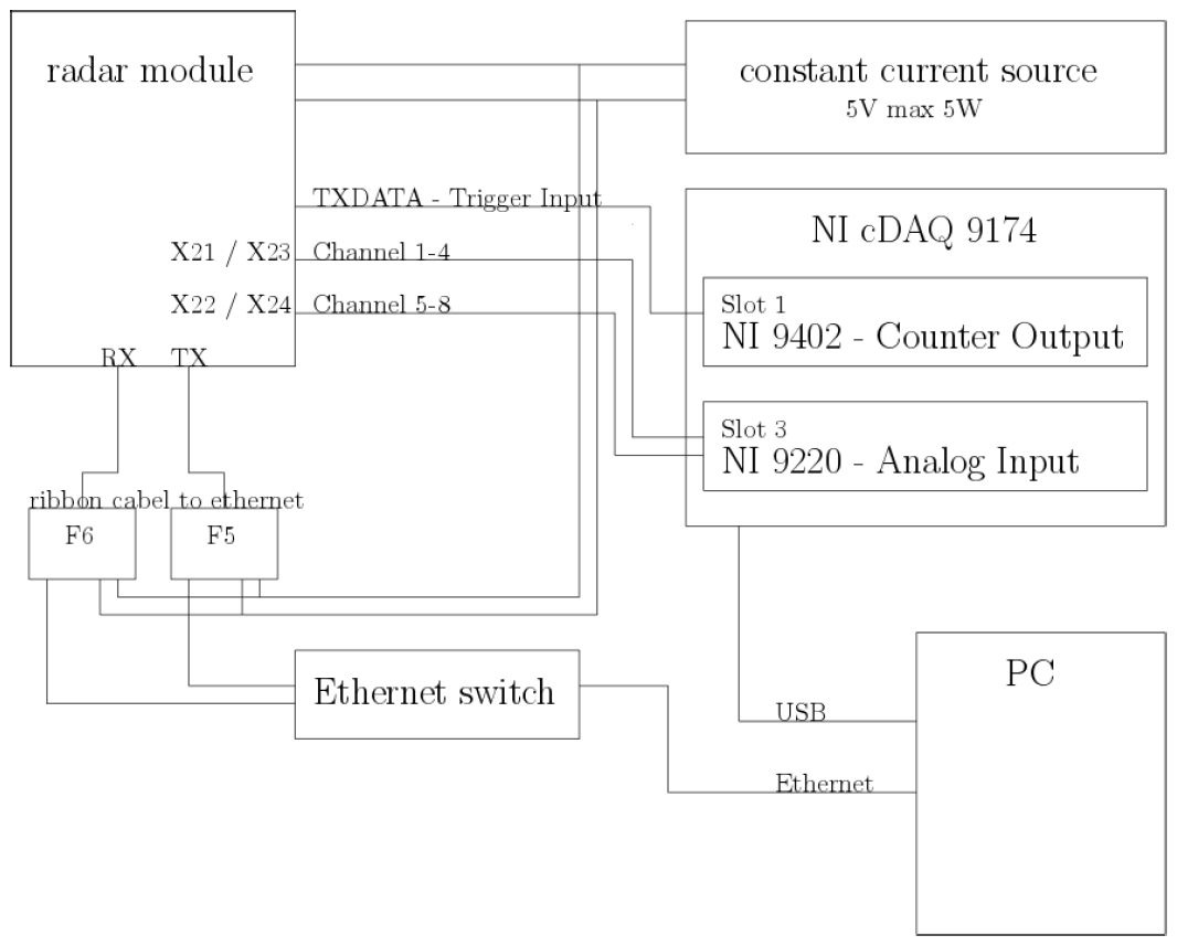
The radar is a FMCW system in the 24 GHz ISM band with two transmit antennas and eight receive channels. The radar is based on a ANALOG DEVICE chip set (ADF5901 and ADF5904) and is developed in the university institution (see Fig. 4) and has been presented in Dirksmeyer et al. (2018). The operation bandwidth is limited to 250 MHz by legal regulation with a transmit power of 20 dBm EIRP. Thus the range resolution is 60 cm. The receive and transmit antennas are leaky wave antennas described in Diewald et al. (2019) with a gain of 13.5 dBi, a half-power beam-width of 17∘ in elevation and a sidelobe level of −10 dB.
The data acquisition is executed by a NATIONAL INSTRUMENTS cDAQ system. The schematic of the the radar and the data acquisition is shown in Fig. 5.

In this section the 2D-Fast-Fourier Transform algorithm is explained to create a 2D-FFT SAR image from the raw radar data. This requires several signal processing steps as shown in Fig. 6. The algorithm applies a FFT to calculate the distance information contained in each echo time signal. Furthermore, the directional information in the phase shift of each measurement is calculated by a second FFT. With the combination of the distance and angle of an object to the radar, the exact position in Cartesian coordinates can be calculated.
3.1 Data representation
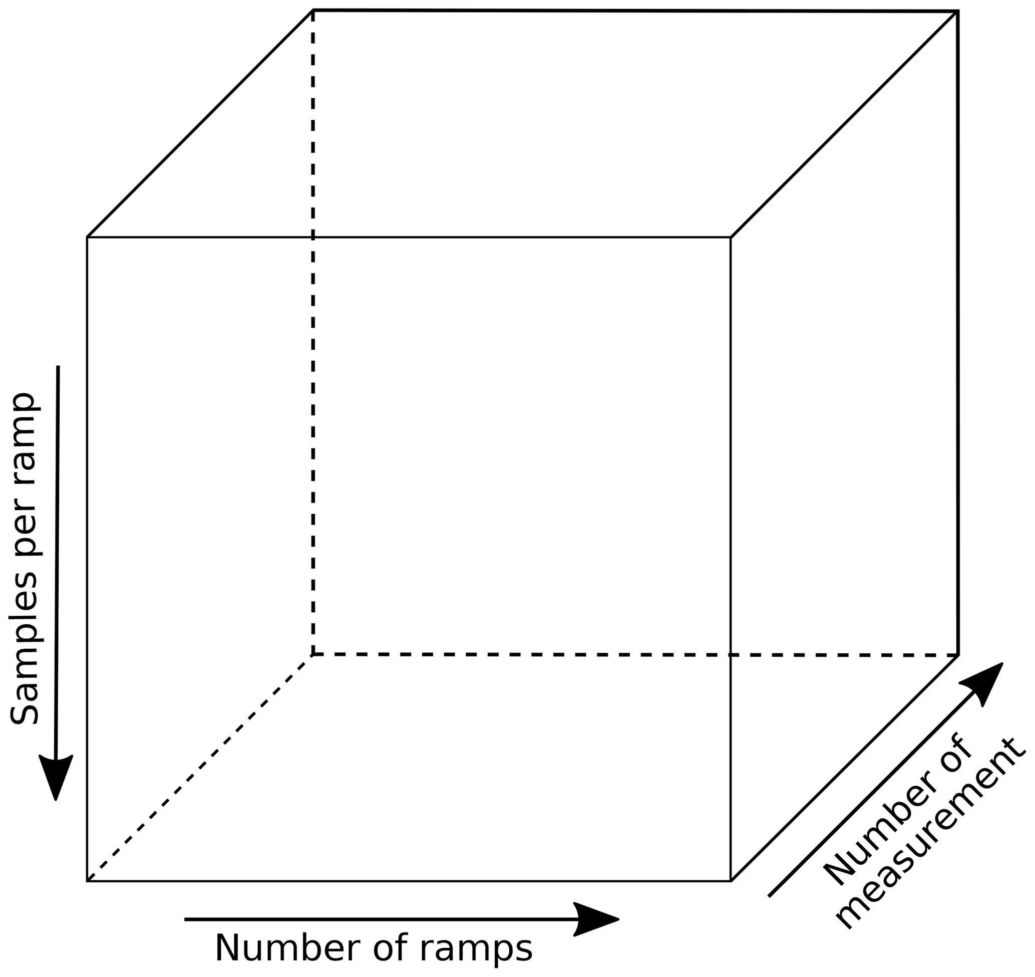
By creating the synthetic aperture the radar transmits several frequency ramps at each position on the axis of the linear drive. In the first step of signal processing the raw data were reshaped into a 3-dimensional cube (Fig. 7) with the dimensions where Ns is the number of samples per ramp, Nr is the number of ramps per measurement point and Nm is the number of measurement points.
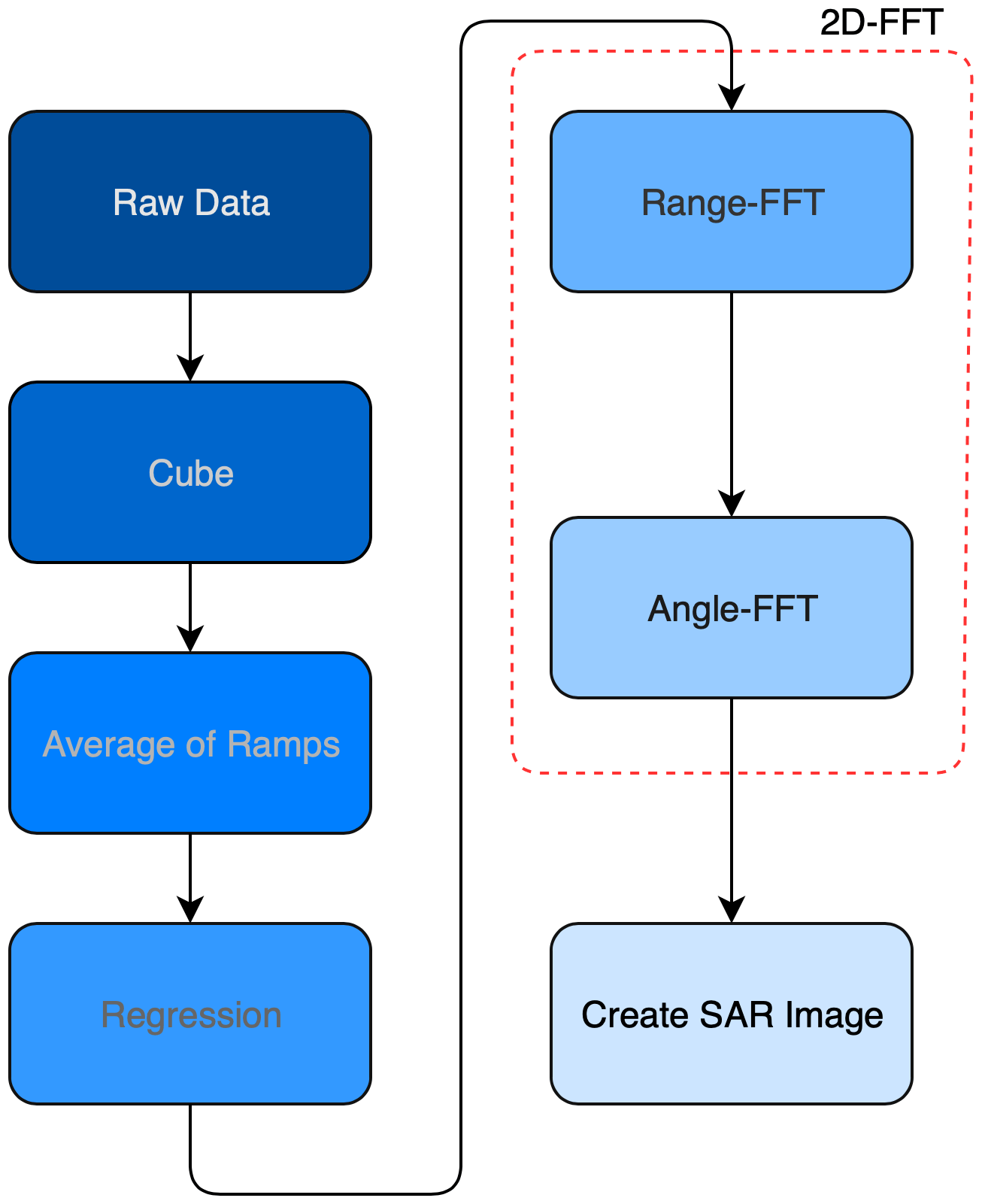
In a second step the mean value is formed over the second dimension of the cube, which reduces the noise and suppresses moving objects in the scenery.
The radar signal is superimposed with a frequency-dependent electronic offset. In a third step the offset is greatly reduced with a linear regression.
3.2 Range-FFT
To reduce the leakage effect and the sidelobes, first a Hamming windows is multiplied with the time domain signal of each ramp. For the range FFT the ramp-averaged time signals are converted into the frequency domain with the digital frequency transformation (DFT) in Eq. (1). The calculation of the DFT is carried out by standard MATLAB functions.
N is the number of measured values on each frequency ramp while x[n] is the nth real-valued voltage signal of the ramp. X[k] is the kth value of the complex-valued frequency domain signal. By the frequency difference Δf the range vector is calculated.
3.3 Angle-FFT
The range-FFT yields a complex-valued matrix with the dimensions . For large distances by a target with R≫LSA the angle estimation can be described as planar wave front with a constant phase shift between each spatial antenna position which is dependend on the incident angle of the target. So the phase shift between two spatial measurement points can be calculate with Eq. (2).
where φ is the phase shift between two subsequent measurements on the linear drive and d is the spatial shift. The azimuthal incidence angle is given by θSA. The complex-valued signal after the range FFT includes the phase information of each measurement. Thus, the phase shift produces sinusoidal values over the imaginary antennas with an angle-dependent frequency fangle. The frequency fangle is calculated over a second FFT in the dimension Nm. As in Sect. 3.2 the signal is windowed by a Hamming window and zero padded to the signal length NFFT,A. By transforming Eq. (2) the angle vector can be calculated by Eq. (3).
For targets with closer distances Eq. (2) is erroneous as the angle θSA changes with each antenna position. Thus, the frequency backprojection algorithm seems to be advantageous in the near range.
3.4 Create SAR image
To create a radar image from the calculated data, a transformation from the cylindrical coordinate system to the Cartesian coordinate system is required. Therefore, the range vector and the angle vector are transformed into the matrices θSA and R.
The Cartesian coordinates matrices X (Eq. 5) and Y (Eq. 6) are calculated.
With the x and y coordinates a radar image is generated. The corresponding logarithmic values from the 2D FFT are displayed in a colour map according to their range, the colour scaling is chosen arbitrarily. Reflective areas are thus displayed in yellow colour and non-reflective areas in blue colour.
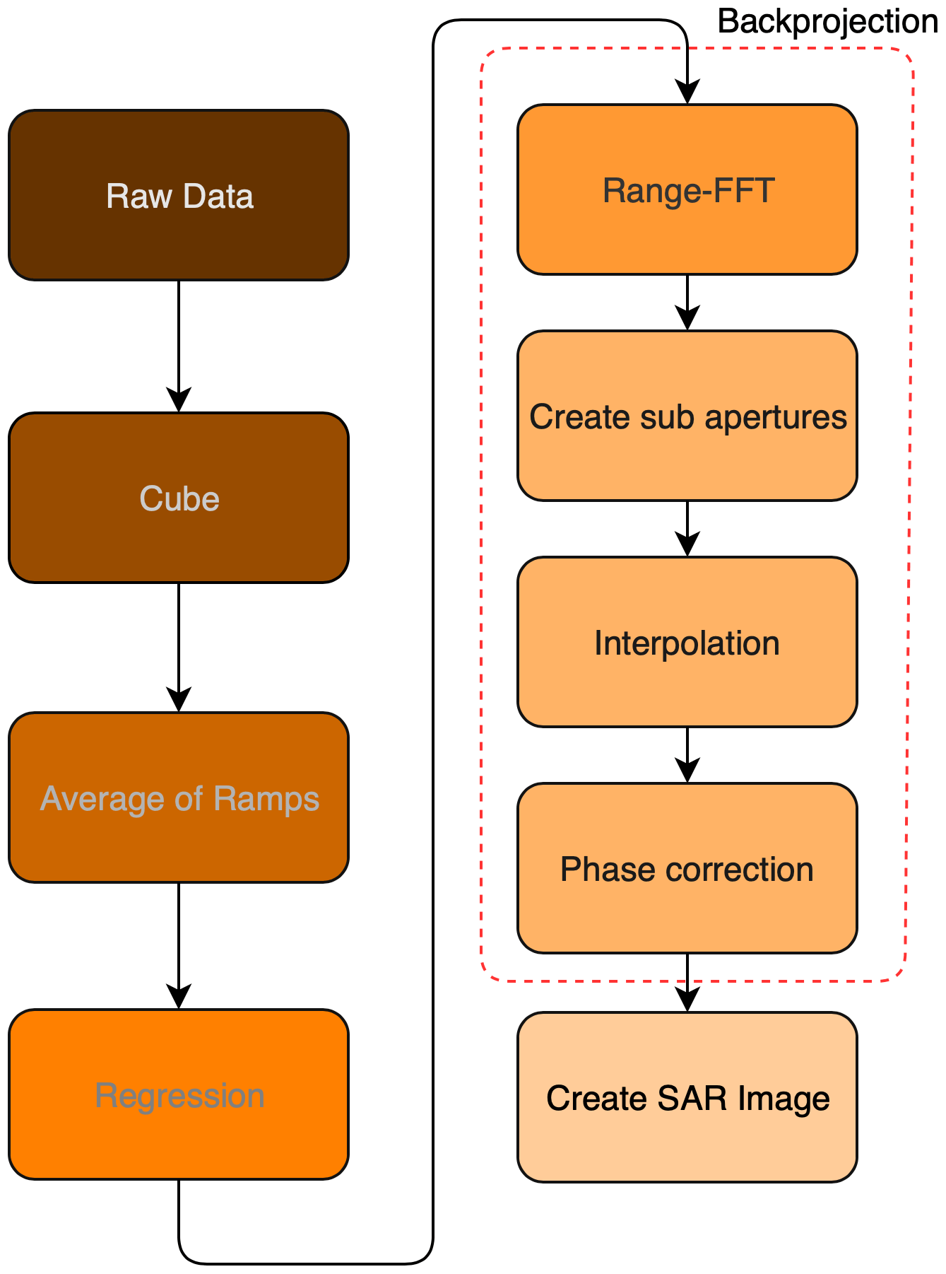
Just like the 2D-FFT algorithm the radar raw data are transformed into a three-dimensional cube, an average of the frequency ramps is performed and a regression is used to calculate the electronic offset. The frequency backprojection algorithm (FBP) creates subapertures from the synthetic aperture and superpose them additively in a manner that an image with M×L pixels is created. Figure 8 shows the signal processing flow of the algorithm.
4.1 Creating subaperture
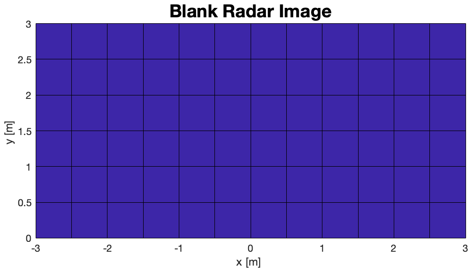
The range FFT is the same as in Sect. 3.2. With Nm measurements, Nm subapertures are created. The subapertures result from the individual radar measurements which together form the synthetic aperture. Each subaperture is projected onto an image grid with M×L pixels in Cartesian coordinates. The discretization in the x and y direction can be chosen freely but should not be coarser than the azimuth resolution (Li et al., 2015). Figure 9 shows an example of an empty image on which the individual subapertures will be projected later on. The image has 12×6 pixels with a discretization of 0.5 m in x and y coordinates. It is crucial how the ROI (Region of Interrest) is chosen, because the amount of data and the computation time increases considerably depending on the size of the area to be mapped.
To project the subapertures onto the image, the distance to the pixels must first be calculated (Eq. 7). Since only a two-dimensional image is generated the z coordinate is a constant value that only represents an offset in the distance.
However, the radar moves over a platform, the distance is slightly different for each single measurement. For a linear movement of the radar in the x direction, the formula changes as follows:
with n∈ℤ.
To project the subapertures onto the image, the complex-valued data must first be interpolated and then superimposed.
4.2 Interpolation
The spectrum is interpolated onto the two-dimensional M×L pixel image. An example of a target range spectrum is shown in Fig. 10. Here the frequency axis was exchanged with the range axis ().

The range resolution is limited to 60 cm due to the bandwidth of the FMCW signal. However, the radar image usually has a significantly higher pixel density. The missing values are thus interpolated complex-valued. Since the time signal is only a finite signal, this corresponds to a rectangular window. Calculating the DFT (Eq. 1) creates a sinc function for the frequencies that occur. After considering that the spectrum consists of one or more sinc functions, a sinc interpolator is used to interpolate. The Sinc interpolator can be implemented by applying zero padding to the time signal before FFT and performing a linear interpolation on the range spectrum.
The interpolation and the superposition of several measurement is shown schematically in Fig. 11.
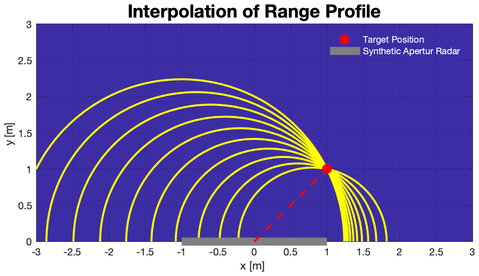
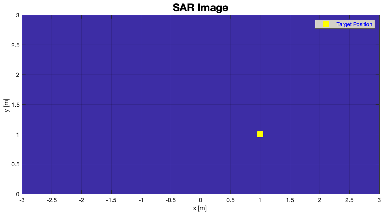
A target is located at . The synthetic aperture is shown in grey on the picture and is located between −1 and 1 m on the x axis and at .
When interpolating, each subaperture will show a shift around the reference point . Each subaperture has a greater or lower distance to the target than the previous or subsequent subaperture. Semicircles are created for each pixel of the coordinate system where applies. When the individual subapertures are superposed the semicircles intersect at one point which shows the exact position of the target. The addition of the subapertures (each semicircle corresponds to a subaperture) increases the intensity at the intersection. The interpolated range spectrum can be specified with Xint[R,m]. R is the range matrix which is calculated from the matrices X and Y (Eqs. 9–10).
According to the DFT, complex-valued data is created that contains phase information. This ensures that the intensity is interfered destructively in places where no targets are and increases for real targets. However, a phase correction is required for this.
4.3 Phase correction
The interpolation also projects the phase onto the image of each subaperture. The phase function can be described by Eq. (11)
The phase of the echo signal depends on the distance r to the target. Considering a subaperture with a target in a distance and a second subaperture with the same target at the phase difference can be described as follows:
Since the subapertures are superposed after the interpolation and the phase changes according to the Eq. (12) for each subaperture, the complex values would not increase but rather decrease. To prevent this the phase is corrected for each pixel. The phase difference is calculated for each image pixel and added to the phase of the interpolated range spectrum of the subaperture.
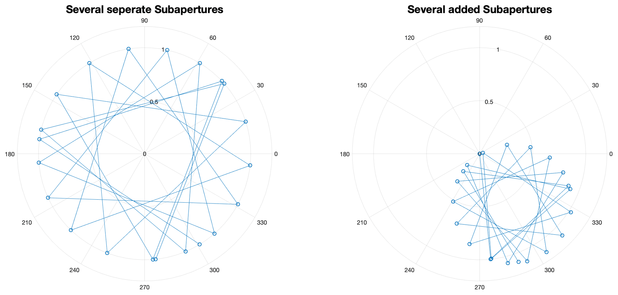
Figure 12 shows the polar plot for a target at a certain distance. The absolute value and phase of the individual subapertures for the same target can be seen in the left plot. The phase changes with each subaperture although the magnitude remains the same. The right picture shows the successive superposition of the subapertures. The absolute values would add up for real data, but for complex data like this, the values will not increase in total no matter how many subapertures were created.
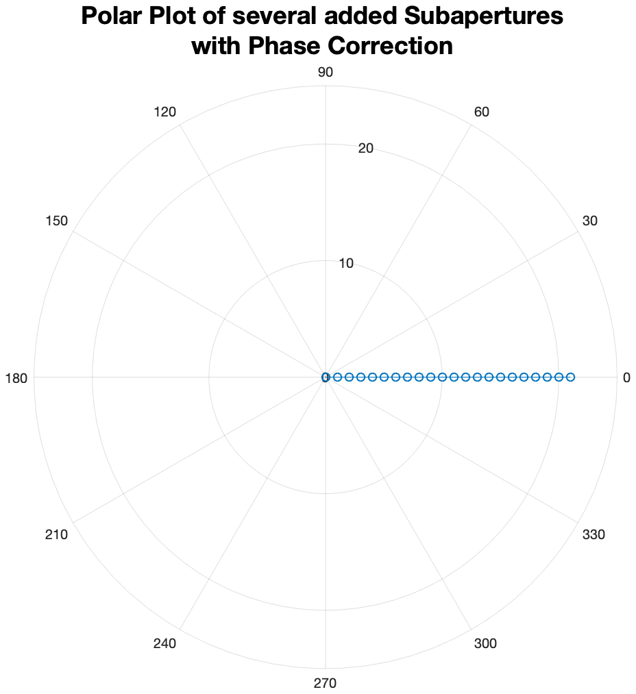
In order to be superposed correctly for the absolute values, the calculated phase ϕ(R) is added to the interpolated phase of each image pixel from the individual subapertures by multiplication with a complex-valued exponential function (Eq. 13).
After the phase correction the absolute value consists of real numerical values, whereby the absolute value add up as shown in Fig. 13. For image pixels where there is no target the phase correction yields a destructive interference and will behave as in Fig. 12 (right). The semicircles disappear and merge into a small point which corresponds to the real target position.
4.4 Create SAR image
After the range spectrum for each subaperture has been interpolated and corrected in phase, the subapertures can be superimposed on a final radar image. With Eq. (14) the M×L pixel image can be calculated with the pixel distance r from the origin and Nm subapertures.
The radar image given in Fig. 14 shwos a blue-yellow blue-yellow gradient the intensities of the backtracked targets at the calculated positions. Yellowish colour areas show high intensities and blue areas show little or no intensities. Sections 5 and 6 show the results of far and near range measurements.
In this section, the 2D FFT and FBP algorithms are applied to the recorded radar data of far range measurements. The far range is meant here with with LSA is the length of the synthetic aperture.
The radar images are superimposed on 2D satellite images from Google Maps and have been compared with optical images which shows the occupancy state of the parking lot. These comparison results are not shown in this publication because it has already been presented in Diewald et al. (2018). In this publication the images of some targets are compared for the two approaches and statements are made about the quality of the images. The colormap scaling of the power is logarithmic and the threshold of the transparency is chosen in this way that the target images shows comparable levels.
Figure 3 from Sect. 2.1 shows the measurement setup and the satellite image of the university parking lot P4. The origin of the x and y axis was placed at the location of the radar unit during the measurement. Since only the area of the parking lot is of interest, only its radar data is evaluated. The optical recording of the satellite image does not correspond to the radar measurement. Therefore the parking lot occupancy shown in the Google images is not equal to the actual occupancy at the time of the radar measurement. The satellite image is for illustration purposes only and helps to evaluate the results. The visible targets of the radar images shown in this chapter are mainly cars from the parking lot.
5.1 Far Range Parking Lot Measurement
The measurement was performed on 15 August 2018. First the radar images from Fig. 17 are compared with each other. The radar image shows a very low occupancy of the parking lots. The pictures seem to differ barely from each other. The reflections (shown in yellow) are in the same positions in both images and are identical with real objects in the scenery (mostly vehicles, street lamps, parking lot gate).
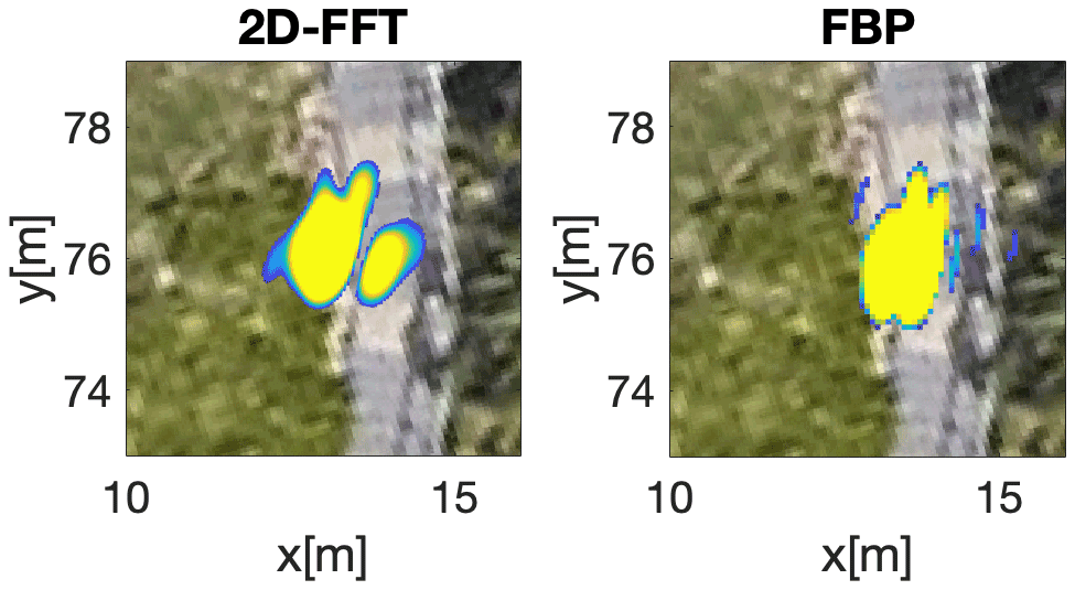
Figure 15Single target zoomed, © Google Maps 2021.
In order to be able to make more precise statements regarding the target contour, images of single targets and multiple targets are zoomed in and the images are compared with each other (Figs. 15 and 16).
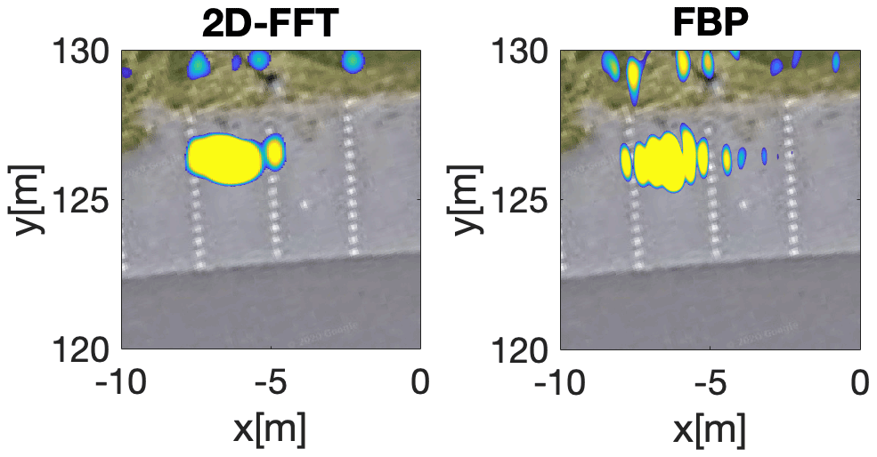
Figure 16Multiple targets zoomed, © Google Maps 2021.
It can be seen that the power values in both images is comparable, the size of the reflected targets remains approximately the same. However, the 2D-FFT radar image shows a smoother, cleaner shape than the FBP.
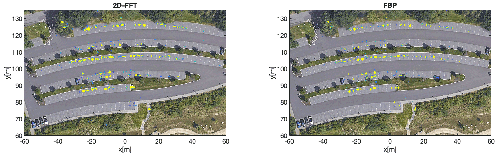
Figure 17Parking lot P4 Trier University of Applied Science satellite image with overlayed radar data, © Google Maps 2021.
There are also some more interferences (small colour spots) in the FBP image. The FBP image looks a bit more pixelated which is also due to the pixel size of the radar image. As in Table 1 No. 1, the 2D-FFT image with 3955×7885 pixels contains significantly more data points than the FBP image with 938×1501 pixels.
In a second radar measurement from 5 June 2018 the parking lot with a high parking space occupancy was recorded. With this the azimuth resolution can be compared well with each other because there are many objects very close together. For the SAR image a step size of d=3 mm was chosen. That are 634 measurements which corresponds to an aperture length of LSA=1.899 m. The comparison in Fig. 18 shows a very good angular resolution. The targets that are close to each other can be better separated. Small gaps between the parking spaces can be seen. This is due to the significantly long synthetic aperture which is decisive for the angular resolution. The FBP algorithm represents more targets than the 2D-FFT algorithm (see range P(8–2,105–106 m)).
5.2 Runtime measurement
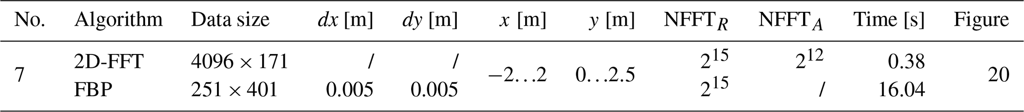
For an appropriate qualitative comparison of the two SAR methods, the runtimes and various other parameters are important, too. The Table 1 shows a list of various parameter specifications and the corresponding qualitative characteristics. The parameters dx and dy each indicate the discretization in x and y direction of the FBP algorithm. The calculated distance range is specified with the parameters x and y. NFFT,R and NFFT,A describe the zeropadding for the distance and the angle respectively. The time indicates how long the respective algorithm requires to calculate the data but the time does not include the plotting process which is often very time-consuming.
Table 1Runtime comparison of 2D-FFT and FBP algorithm in far range.

Basically, it can be seen that FBP requires significantly more time than the 2D-FFT algorithm. However, the result data are clearly smaller than with the 2D-FFT. If the ROI reduces the calculation time for the FBP algorithm is reduced, too while the processing time for te 2D-FFT method stays nearly constant. With the FBP, only the area that is to be displayed is authorized. With the 2D-FFT, however, the complete range up to the area to be displayed must be calculated. Decisive for the calculation time of the FBP is the discretization in x and y direction and the area to be displayed (number of pixels). For the 2D-FFT algorithm, the maximum distance range and the range zero padding are important for the running time. The main reason for the long runtimes of the FBP is the type of calculation. In the FBP, a subaperture is created for each shift of the radar antenna, which are interpolated individually to an M×L pixel image and then added together (Sect. 4). This is a much higher computational effort than performing an FFT in two dimensions which is a very fast operation anyway. In the far range there are no significant qualitative differences between the two algorithms. Due to the long runtime of the FBP algorithm compared to the 2D-FFT, the use of the 2D-FFT is to be preferred. If the runtime is not important, the FBP algorithm should be chosen, as it produces a slightly better radar image. The parameter settings from measurement 5 of the table offer a good compromise between runtime and image quality of both algorithms.
The computer used for all calculations for the measurements performed in Table 1 has the following system properties:
-
Operating system: macOS Catalina
-
Processor: 2.8 GHz Dual-Core Intel Core i5
-
Memory: 8 GB 1600 MHz DDR3
-
Video card: Intel Iris 1536 MB
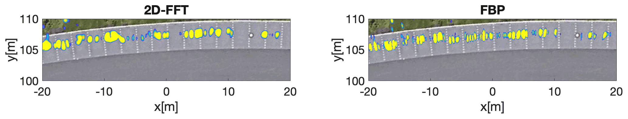
Figure 18Parking lot with 2D-FFT and FBP, © Google Maps 2021.
In order to get a good comparison for the near range, SAR measurements were performed at a distance of 1–12 m. The near range is for R≤20 m. The targets (corner reflectors) were measured at different positions in an anechoic chamber equipped with absorber foam. Both algorithms (2D-FFT and FBP) are applied to the measurement data and compared with each other. For each measurement there are different runtimes measured that occurs by different parameters which can be seen in Table 2. The targets of the radar measurements are implemented as corner reflectors with effective radar cross sections as follows:
-
Corner reflector 1: σ=0.13 m2
-
Corner reflector 2: σ=1 m2
-
Corner reflector 3: σ=1 m2
-
Corner reflector 4: σ=0.13 m2
-
Corner reflector 5: σ=35 m2
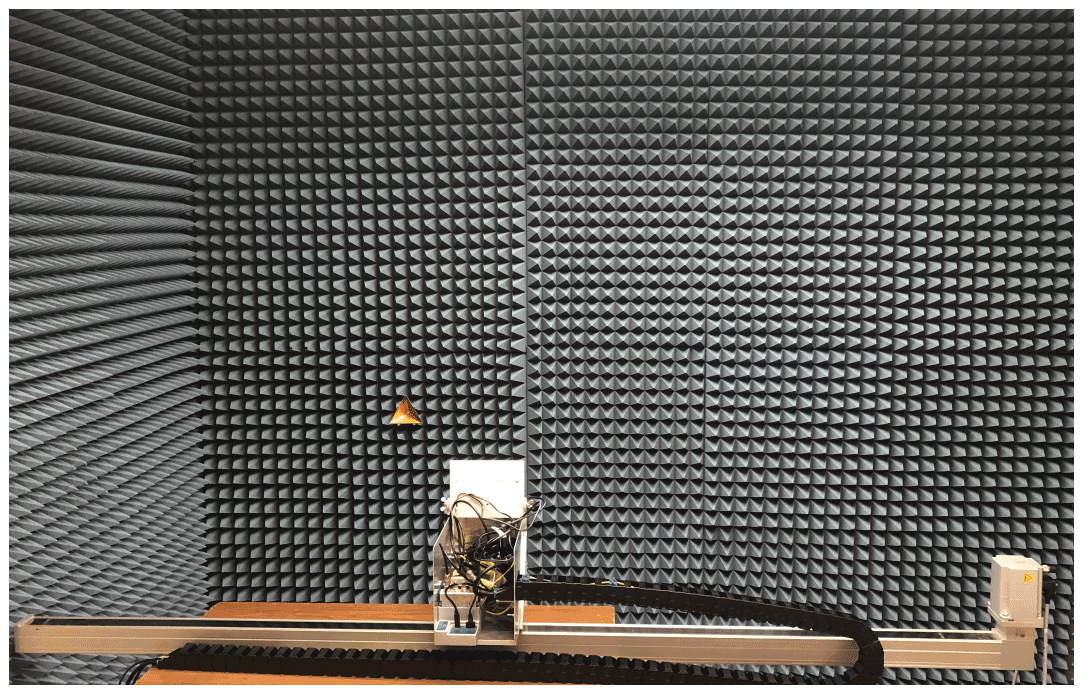
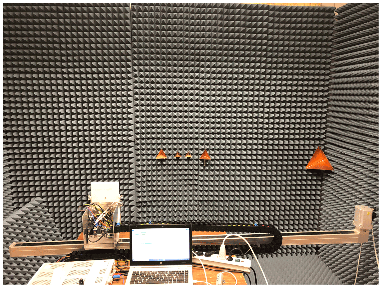
The measurement setup shown in Fig. 19, shows the measuring chamber with the absorber foams and the SAR system implemented on the linear drive. The foam absorbs the electromagnetic waves and ensures that no reflections of the walls disturb the measurements. The corner reflector, on the other hand, ensures a particularly good reflection whereby all incoming electromagnetic waves are reflected back at the incident angle. This measurement setup allows very accurate measurements to be made with almost ideal targets and almost no reflection from other interfering elements. In the subsequent measurements the targets were set at the same height as the radar unit (z=0). The x axis responds to the path from left to right, which also means that the displacement of the radar unit also takes place in x direction. The y axis corresponds to the distance in the plane between the SAR and the targets. The targets were fixed at different positions and measured simultaneously. For each measurement the x and y coordinates to the reference point P(0,0) of the SAR were roughly measured with a tape measure. Thus, the values may differ by ±5 cm. All coordinates of the corner reflectors are indicated with where Ci with the index stands for the different reflectors. The coordinates resulting from the radar image are specified with , where i is the corner reflector number.
6.1 Near range with five corner reflectors
A measurement with all five corner reflectors was performed. Figure 21 shows the measurement setup and Fig. 20 shows the results. The corner reflectors were attached to the following positions: , , , , . In this measurement the y distance to the radar was reduced to 90 cm and the two small corner reflectors C1 and C4 were placed in the middle with a distance of only 10 cm to each other. The next larger reflectors C2 and C3 are placed to the left and right of the smaller reflectors with a distance of 15 cm. The large corner reflector C5 is located on the far right corner.
The left radar image, which contains the 2D-FFT data, shows a merging of the four middle targets that have their intensity maximum at . The right target are by which have a very large deviation from the given position.
The right radar image shows the output of the FBP algorithm. The intensity maxima of the targets at the narrowest points are as follows: , , , and . The four middle targets can be separated easily. The distances between the middle reflectors are calculated:
These results speak for a very high accuracy of the FBP compared to the 2D-FFT algorithm, as they are very close to scale.
Table 2Runtime comparison of 2D-FFT and FBP algorithm in near range.

6.2 Runtime measurement
Table 2 shows a set of parameters of near range measurements and the specified calculation time of the algorithms. Depending on set parameters, the runtimes vary extremely. In general, the 2D FFT algorithm is 25 to 150 times faster than the FBP algorithm. As with far range measurements, the propagation time of the 2D-FFT is dependent on the length of the signal, i.e. zero padding. With FBP, the discretization in x and y direction is decisive for the runtime. The discretization should be selected so that the pixel size is significantly smaller than the resolution. If the runtime is important, a discretization of 10 cm also gives good results, but with a somewhat coarser pixel size. If the discretization is even coarser, the result will be inaccurate and the targets will be harder to recognize. The optimal settings are a compromise between runtime and pixel size. The results of measurement No. 3 and 4 from the table give very good results with a relatively short runtime. A discretization of 1 cm was chosen, which results in runtimes below 10 s and still gives a good pixel size. Measurement No. 9 and 10 result in a very long run time, because a much larger range is calculated. Here one could consider to increase the discretization a bit.
The 2D-FFT algorithm is not critical of the runtime. However, a zeropadding of more than 215 does not provide a noticeable improvement of the radar image.
A Radar System implemented on a linear drive as a Synthetic Aperture Radar is a good way to learn and understand the underlying SAR methodology. It also improves the angular resolution in comparison to classical digital beamforming and MIMO radars to such an extent that it can be used for imaging of parking lots or even indoor areas which provides an educational success by learning these methods. The near range and far range data examined here and the comparison of the 2D-FFT algorithm with the FBP algorithm bring out the qualitative properties of these two SAR processing algorithm. The results from the far range measurement of the university parking lot from Sect. 5 show that the two algorithms produce approximately equally good radar images. The FBP has a slightly better resolution which makes it easier to separate objects. The 2D-FFT, on the other hand, delivers smoother images with a much shorter runtime in spite of its higher pixel density. Unfortunately targets overlap more often due to the slightly poorer angular resolution caused by the assumption of a constant azimuth angle for each individual measurement on the linear axis.
The near range measurement from Sect. 6 shows the opposite effect. By using corner reflectors and a measuring chamber equipped with absorber foam almost ideal measuring conditions could be created. The results show a clear advantage of the FBP algorithm over the 2D-FFT. The FBP images show a very good azimuth resolution, with the reflections of the corner reflectors shown in x-shape. The narrow points (cross point) show almost exactly the coordinates previously determined with a measuring tape. In addition, even several reflectors placed next to each other at a distance of 10–15 cm can be clearly distinguished. Starting point for the exact coordinates are the maximum intensities calculated by the respective algorithm.
The 2D-FFT algorithm shows very bad results in the near range because targets that are close to each other merge together and also the coordinates from the measured targets have large deviations from the real position. The targets are generally displayed wider and larger because the 2D-FFT algorithm pulls them apart due to the missing consideration of the displacement. The properties of the corner reflectors enable the FBP algorithm to calculate the target position with centimetre accuracy due to the azimuth resolution. The limited range resolution of 60 cm does not play any role here since the narrow part of the x-shaped display represents the exact position of the target. For targets with R≫LSA this effect is not observed. The runtimes of both algorithms are very far apart. The 2D-FFT computation time is a fraction of the FBP runtime. The results show that the runtime of the FBP algorithm depends mainly on the number of individual measurements, i.e. subapertures. The runtime of the 2D-FFT depends mainly on the number of the selected zero padding.
The resolution of both algorithms is dependent on the length of the aperture LSA and not on the step size between the individual measurements. However, the condition must be fulfilled.
In conclusion, it can be said that both algorithms provide good results depending on the field of application. It is recommended to use only the FBP algorithm in the near range, because only this algorithm gives good results there. In the far range, both algorithms can produce very good radar images, whereby the recommendation here is to use the 2D-FFT algorithm as this has a runtime up to 150 times shorter than the FBP algorithm. If the near and far range have to be covered, the FBP algorithm should be selected.
The code was written by Jonas Berg in his master thesis and the code is his proprietary. Nevertheless the university institution is authorized to deliver the code to interested people upon their request at diewald@hochschule-trier.de
No data sets were used in this article.
JB worked on the project as Master student at the Laboratory of Radar Technology and Optical Systems, he programmed the signal processing and evaluated the results. SM developed the 24 GHz radar system. AD is the head of the institution, he developed the radar system, gave the initial idea and developed the signal processing, organised the team and wrote this publication.
The contact author has declared that neither they nor their co-authors have any competing interests.
Publisher's note: Copernicus Publications remains neutral with regard to jurisdictional claims in published maps and institutional affiliations.
This article is part of the special issue “Kleinheubacher Berichte 2020”.
This paper was edited by Madhu Chandra and reviewed by S. Hussian Kazimi and one anonymous referee.
Diewald, A. R., Berg, J., Dirksmeyer, L., and Müller, S.: DBF and SAR Imaging Radar for Academic Lab Courses and Research, European Microwave Conference (EuMC), 25–27 September 2018, Madrid, Spain, 48, 2018. a
Diewald, A. R. and Müller, S.: Design of a six-patch series-fed traveling-wave antenna, 2019 IEEE-APS Topical Conference on Antennas and Propagation in Wireless Communications (APWC), Granada, Spain, https://doi.org/10.1109/APWC.2019.8870368, September 2019. a
Dirksmeyer, L., Diewald, A. R., and Müller, S.: Eight Channel Digital beamforming Radar for Academic Lab Courses and Research, 19th International Radar Symposium (IRS), Bonn, Germany, https://doi.org/10.23919/EUMC.2018.8541400, June 2018. a
Google: Google Maps, available at: https://www.google.com/maps, last access: 17 December 2021. a
Gorham, L. A. and Moore, L. J.: SAR image formation toolbox for MATLAB, Proc. SPIE 7699, Algorithms for Synthetic Aperture Radar Imagery XVII, 769906, https://doi.org/10.1117/12.855375, 18 April 2010. a, b
Li, Z., Wang, J., and Liu, Q. H.: Frequency-Domain Backprojection Algorithm for Synthetic Aperture Radar Imaging, IEEE Geosci. Remote S. Lett., 12, 905–909, https://doi.org/10.1109/LGRS.2014.2366156, 2015. a
Moreira, A., Prats-Iraola, P., Younis, M., Krieger, G., Hajnsek, I., and Papathanassiou, K. P.: A Tutorial on Synthetic Aperture Radar, IEEE Geosci. Remote S. Mag., 1, 6–43, https://doi.org/10.1109/MGRS.2013.2248301, 2013. a
Ulander, L. M. H., Hellsten, H., and Stenstrom, G.: Synthetic-aperture radar processing using fast factorized back-projection, IEEE T. Aerospace and Electronic Systems, 39, 760–776, https://doi.org/10.1109/TAES.2003.1238734. a
Wolff, C.: Radar Basics, available at: https://www.radartutorial.eu/20.airborne/ab08.en.html, last access: 17 December 2021. a, b, c, d, e
- Abstract
- Introduction
- Synthetic aperture radar
- 2D-Fast-Fourier Transform algorithm
- Frequency Backprojection Algorithm
- Comparison of the FBP and 2D-FFT algorithm based on far range measurements
- Comparison of the FBP and 2D-FFT algorithm based on near range measurements
- Conclusion
- Code availability
- Data availability
- Author contributions
- Competing interests
- Disclaimer
- Special issue statement
- Review statement
- References