Potentials of the Application of the Electrical Transmission Line Theory for Thermal Investigations on Cables

In this contribution, similarities and differences between electrical and thermal effects on cables are investigated. In the electrical transmission line theory, a wide variety of methods is known to describe the voltage and current along cables. The potential for the adaption of some of those methods to thermal problems is discussed. Exemplarily, for an unshielded single cable, an analytical solution based on the Laplace transform and an approach based on cascaded equivalent circuits are compared with a numerical reference solution and measurement results.

1 Introduction

Because of the rising complexity of electric systems, more and more cables are necessary for the power supply of different components. Especially in safety-critical applications, high demands concerning reliability and electrical resilience are present (Horn et al., 2018). On the other hand, electrical systems become more compact which complicates the heat transport and leads to higher cable temperatures. Derating of the temperature sensitive insulation materials can lead to critical failures, and monitoring of cable temperatures is essential to prevent the insulation from damages by too high temperatures.

During the lifetime of a cable, temperatures might change in a wide range, especially in mobile systems. Dimensioning of insulation geometry and materials is mostly done by calculations based on the heat transfer differential equation. Parameter sets are based on worst case assumptions (Wright and Newberry, 2008). Due to nonlinear material parameters the equation is nonlinear and mostly numerical methods are used (He et al., 2013) leading to high calculation effort and low transparency.

To protect cables under operation, often melting fuses are used. Those do not consider the actual cable status, but trigger depending on the temperature of the melting wire. This often causes over-dimensioned cables. Also, automated resetting is not possible for melting fuses. That is why electronic smart fuses (Tian et al., 2019) are more and more applied as exemplarily shown for a vehicular application in Fig. 1.

Figure 1 Smart fuse in an exemplary vehicular application.

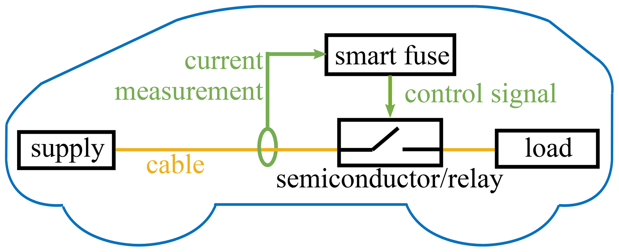
Especially in safety-critical environments, where overload situations should be tolerated as far as possible, and a hard interruption of the power supply has to be avoided, the use of smart fuses may drastically enhance the reliability of the complete system. A wide range of applications from automated driving applications or industrial applications to the use in personal equipment is possible. Based on a thermal model of the cable and current measurements, the cable insulation temperature is calculated in real time and a semiconductor or a relay is used to interrupt the circuit in case of too high temperature. Currently, the numerical calculations require powerful computing systems. To enable an implementation on low cost and energy efficient microcontrollers, more computational efficient thermal cable models are necessary.

Electrical signal propagation has been intensively investigated during the last decades and many powerful methods have been developed based on transmission line (TL) theory for a conductor pair or multiconductor transmission line (MTL) theory for many conductors. The research is still going on.

In this contribution, the adaption of methods from the electrical TL theory to the thermal domain is investigated. In Sect. 2, the state of the art concerning thermal cable models is briefly presented followed by an introduction to the electrical TL theory in Sect. 3. In Sect. 4, similarities and differences between electrical and thermal effects on cables are examined. The potential for the adaption of methods known from the electrical TL theory to describe thermal effects on cables is shown in Sect. 5 using an example: for an unshielded single cable, two methods based on known electrical methods are validated using a numerical reference solution and measurement results.

2 Thermal cable models

In cables, all three well known heat transport mechanisms are important: in the cable itself, mainly heat conduction dominates, described by Fourier's law. The coupling to the environment is dominated by radiation and convection. Considering all three effects, an inhomogeneous nonlinear partial differential equation or even a system of those equations is necessary and general analytical solutions are hard to find.

For thermal investigations on homogenous cylindrical cables, two major directions for the heat flow are distinguished: the axial direction along the cable and the radial direction transversal to the axial direction. Often, the heat flow in the radial direction is considered as dominant, which is a valid assumption for long cables without relevant boundary effects. For example, in Hoffer (1978) and Ilgevicius (2004) only the radial heat flow is considered. In many practical applications, cable contacts heat up or cool the cable. Especially for short cables, this highly influences the cable temperature close to the contacts and the axial heat flow cannot be neglected.

Often, numerical methods like FEM are used as e.g. in Fu et al. (2018) and He et al. (2013). In those methods, the 3D geometry of the cable structure is discretized and the corresponding equations are solved. Those approaches cause massive calculation effort, and, therefore, take a long time. Faster solutions can be found for rotational-symmetric configurations, when just a 2D plane of the complete structure needs to be discretized. Also, calculating only the radial or the stationary temperature distribution (Dai et al., 2014; Loos et al., 2014; Sedaghat et al., 2018) reduces the numerical calculation effort, as dependencies in the partial differential equation vanish and a lower number of elements needs to be taken into account. As in many practical cases, the transient temperature development is searched, these easier stationary solutions often cannot be applied. Contrary to numerical calculations analytical methods can provide solutions in short time, but then restrictions for the environmental conditions and simplifications are necessary.

Other approaches model the cable configuration as a thermal network. Like in the electrical domain equivalent circuits are used for modelling. Holyk et al. (2014), Lauria et al. (2018), Lei et al. (2010), Olsen et al. (2013), and Zhan et al. (2019) considered only the radial heat flow. If axial heat flow is needed, stationary solutions are well known, for example in Rickman and Iannello (2016). Approaches that model the transient axial heat flow are rarely presented. One example is given by Önal and Frei (2018) where cascaded network models are used, that need numerical techniques for computation.

3 Electrical cable models

Electrical cable models were examined for more than one hundred years by now (Paul, 2008). Beginning with simple single cables, more and more complex cable arrangements were evaluated, and the multiconductor transmission-line (MTL) theory was established (e.g. Achar and Nakhla, 2001; Antonini et al., 2013; Paul, 2008). The basic model for an MTL arrangement is shortly presented here. An infinitesimally short cable segment can be modelled using an equivalent circuit (Paul, 2008). From this equivalent circuit, using Kirchhoff's laws, a system of coupled partial differential equations is derived:

$$\begin{array}{}\text{(1)}& \begin{array}{rl}& {\displaystyle \frac{\partial }{\partial z}}\mathit{U}(z,t)=-{\mathbf{R}}^{\prime }\mathit{I}(z,t)-{\mathbf{L}}^{\prime }{\displaystyle \frac{\partial }{\partial t}}\mathit{I}(z,t),\\ & {\displaystyle \frac{\partial }{\partial z}}\mathit{I}(z,t)=-{\mathbf{G}}^{\prime }\mathit{U}(z,t)-{\mathbf{C}}^{\prime }{\displaystyle \frac{\partial }{\partial t}}\mathit{U}(z,t).\end{array}\end{array}$$

Substituting one equation into the other leads to the set of hyperbolic partial differential equations just for the voltages:

$$\begin{array}{}\text{(2)}& \begin{array}{rl}{\displaystyle \frac{{\partial }^{\mathrm{2}}}{\partial z^{\mathrm{2}}}}\mathit{U}(z,t)& -{\mathbf{L}}^{\prime }{\mathbf{C}}^{\prime }{\displaystyle \frac{{\partial }^{\mathrm{2}}}{\partial t^{\mathrm{2}}}}\mathit{U}(z,t)-\left({\mathbf{L}}^{\prime }{\mathbf{G}}^{\prime }+{\mathbf{R}}^{\prime }{\mathbf{C}}^{\prime }\right){\displaystyle \frac{\partial }{\partial t}}\mathit{U}(z,t)\\ & -{\mathbf{R}}^{\prime }{\mathbf{G}}^{\prime }{\displaystyle \frac{{\partial }^{\mathrm{2}}}{\partial z^{\mathrm{2}}}}\mathit{U}(z,t)=\mathbf{0}.\end{array}\end{array}$$

Its solution, the vector U(z,t), describes the development of the voltages along the cables depending on the time t and the spatial coordinate z, I(z,t) are the corresponding currents. The matrices R^′, L^′, G^′ and C^′ are built up from the equivalent circuit.

A huge number of solution approaches of this general problem was developed in the past (see for example Achar and Nakhla, 2001; Antonini et al., 2013; Paul, 2008). Several numerical solutions as finite differences in the time domain (Orlandi and Paul, 1996) or recursive algorithms (Lin and Kuh, 1992) but also many analytical solutions exist for different application scenarios. Often, transformations for example into the Laplace domain (Al-Zubaidi R-Smith and Brancík, 2016; Nuricumbo-Guillén et al., 2018) are applied to find solutions. To uncouple the differential equations, the similarity transform (Lombardi et al., 2018) can be used. As often very complex terms appear, methods for model order reduction (Spina et al., 2014) are applied to reduce the complexity of the resulting formulations and enable further calculation steps. From (explicit) solutions for special cases as homogenous lossless lines to generalizations as for example the inclusion of nonlinear cable parameters (Wang et al., 2019; Zeng and Wong, 1996), a wide variety of methods was explored in the past. The research is still going on. Currently, for example inhomogenous or buckling lines and statistical laying conditions are under investigation (see exemplarily Kasper and Vick, 2019; Sekine et al., 2020).

4 Comparison between the electrical and thermal domain

As in the electrical transmission-line (TL) theory many methods were developed over the years, it is of scientific interest whether the methods can be transferred to thermal problems. This is discussed in this section.

4.1 The thermoelectric equivalent

Electromagnetic effects are based on the behavior of electrical charges q. Likely charges reject each other. On the elemental level, electrical charges are discretized as multiples of the elementary charge. As this elementary charge is very small, on a macro level, this discretization can be neglected. Then, a continuous charge density ρ can be used to describe the charge distribution quite exactly. Without external excitations, this charge density tends to a uniform distribution in space resulting in a constant volume charge density. An equivalent behavior can also be found in the thermal domain: a temperature difference leads to balancing effects resulting in a uniform temperature distribution. Elementarily, the temperature of a medium is characterized by the middle velocity respectively the kinetic energy of the molecules. Analogously to the electrical volume charge density, that tends to a uniform distribution, in the thermal domain, an energy density ρ_th is given. Therefore, thermal “charges” q_th are energy portions. As there is no negative energy, negative thermal charges or charge densities do not exist. This is one elemental difference between electrical and thermal charges. Integrating over the charge density gives the charge for a specific volume in both domains.

The electrical current I is the charge quantity, that passes a given cross section per time. It can be characterized as effect or through quantity. Equivalently, the heat flow P is the energy that passes a given cross section per time.

In the electrical domain, the electrical scalar potential φ and the electrical voltage U are related closely. The potential is the more physical quantity. Physically, a potential describes the ability of a conservative force field to perform work. For the electrical scalar potential this is about shifting charges. The electrical potential is a characteristic of the space itself and can be defined for each point even if there is no matter or charge at the specific point. In the thermal domain, the equivalent quantity is the temperature T. As a temperature always needs matter to be defined, here, electrical and thermal domain differ. The electrical voltage between two points in space is the difference between the potentials of those two points. This voltage can be characterized as cause or across quantity. Therefore, a constant offset does not change the physical behavior, so an offset can be chosen arbitrarily. A fixed reference potential can be defined. All other potentials then refer to this reference. In the thermal domain, equivalently, a reference temperature can be chosen. As the lowest physically possible temperature is the absolute zero point, temperatures below this point cannot appear. Unlike, the electrical scalar potential can have any value.

Energy minimization is a physical basic principle. That is why electrons tend to move towards points with lower potential. Different potentials lead to a voltage between two points and therefore cause a force on charged particles, that leads to a current between these two points, as long as a path with finite resistance exists. The most popular case is a current through a conductor. The ratio between the voltage and the current describes the resistance that the medium sets against this charge movement. Analogously, heat conduction can be modelled: along a medium, thermal charges (energy) move from places with higher potential (temperature) to places with lower potential. Again, the resistance is the ratio between the temperature difference and the heat flow.

Even the calculation formulas for the resistances for special geometries are quite similar: for a cylinder of length l and cross section A, the axial electrical resistance R and the corresponding thermal resistance R_th are calculated via

$$\begin{array}{}\text{(3)}& R={\displaystyle \frac{l}{\mathit{\sigma }A}},R_{\mathrm{th}}={\displaystyle \frac{l}{\mathit{\lambda }A}}\end{array}$$

with the electrical (σ) respectively thermal (λ) conductivity. Also, the radial resistances for a cylindrical shell with the inner radius r₁ respectively outer radius r₂ are

$$\begin{array}{}\text{(4)}& R={\displaystyle \frac{\ln \left(\frac{r_{\mathrm{2}}}{r_{\mathrm{1}}}\right)}{\mathrm{2}\mathit{\pi }\mathit{\sigma }l}},R_{\mathrm{th}}={\displaystyle \frac{\ln \left(\frac{r_{\mathrm{2}}}{r_{\mathrm{1}}}\right)}{\mathrm{2}\mathit{\pi }\mathit{\lambda }l}}.\end{array}$$

Additionally, in the thermal domain, the resistance for a surface A with the heat transfer coefficient α is calculated via

$$\begin{array}{}\text{(5)}& R_{\mathrm{th}}={\displaystyle \frac{\mathrm{1}}{\mathit{\alpha }A}}.\end{array}$$

The current density J in the electrical domain respectively $\dot{\mathit{q}}$ in the thermal domain is calculated via a multiplication of the gradient of the potential (temperature) with the conductivity. Then, the current through a given cross section is the integral over the current density. From the charge conservation, the continuity equation follows, that relates the electrical charge density and the current density. Analogously, in the thermal domain, energy conservation leads to an equivalent formulation.

Due to energy conservation, the energy imprinted on a structure splits up in a part that is preserved in the volume and heats up the structure and a part that leaves the structure via its surface. For the heat storage in the medium, capacitances are necessary. In the electrical domain, capacitances are used to characterize the capability of storing charges. Generally, this describes a property between two conductive structures. The charge +Q is applied to the one structure, the charge −Q to the other one. The capacitance C then describes the connection to the voltage between both structures.

$$\begin{array}{}\text{(6)}& C={\displaystyle \frac{Q}{U}}\end{array}$$

To find the charge Q, an integration over a surface that fully includes one of the structures is necessary. For the voltage U, an integration along a path between the two structures needs to be calculated. So, this property depends on the material between the structures and the geometry. The most typical example for an electrical capacitance is a parallel-plate capacitor, which is a structure of two electrically conducting parallel structures that are insulated from each other. In the thermal domain, there is no equivalent to that. Here, capacitances fulfil a different task. Generally, again, the storage capability of energy (corresponding to the electrical charge) is described. In the thermal domain, a single structure is sufficient to define that property. The thermal capacitance deals with the question how much energy needs to be put into a structure to generate a defined temperature increase. As the temperature is measured relatively to the fixed reference temperature, the capacitance refers to this reference as well. The thermal capacitance C_th of a structure is a property of a single body, that depends on its material and volume, but not on the geometry. For the calculation, the specific heat capacity c_m respectively the volumetric heat capacity c_V is multiplied with the mass m respectively volume V of the observed structure:

$$\begin{array}{}\text{(7)}& C_{\mathrm{th}}=c_{V}V=c_{m}m.\end{array}$$

A thermal capacitance always refers to the reference and cannot be placed between two structures (Kipp, 2008). Capacitances are used to calculate the temperature development along time:

$$\begin{array}{}\text{(8)}& T\left(t\right)={\displaystyle \frac{\mathrm{1}}{C_{\mathrm{th}}}}\underset{\mathrm{0}}{\overset{t}{\int }}P\mathrm{d}\mathit{\tau }+T_{\mathrm{0}}.\end{array}$$

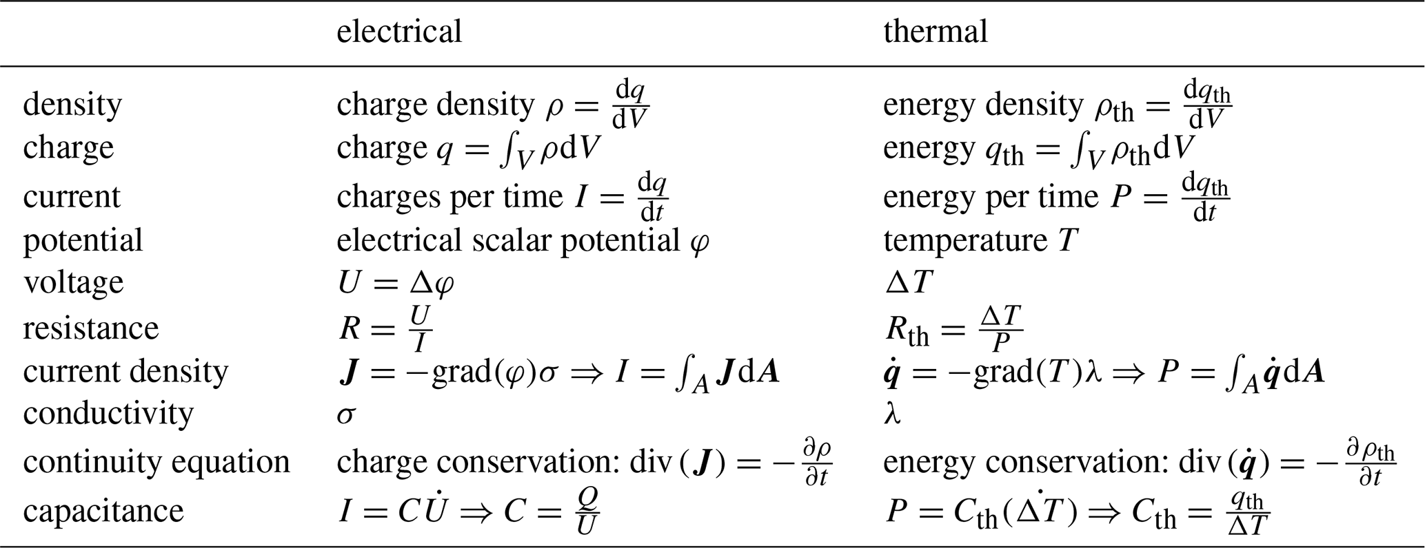
There is no thermal equivalent to the electrical inductivity. An overview over the presented equivalences is given in Table 1.

Table 1 Overview over equivalences between the electrical and thermal domain.

4.2 Derivation of thermal equivalent circuits

Equivalent circuits can generally be used to describe systems based on conservation laws. So, based on the equivalences between the electrical and thermal domain, thermal equivalent circuits can be derived to describe thermal effects on different structures analogously to the electrical version. In Fig. 2, this is shown exemplarily for a segment of length l of an infinitely long homogeneous single wire with insulation.

Figure 2 Equivalent circuit for a cable segment of a single cable.

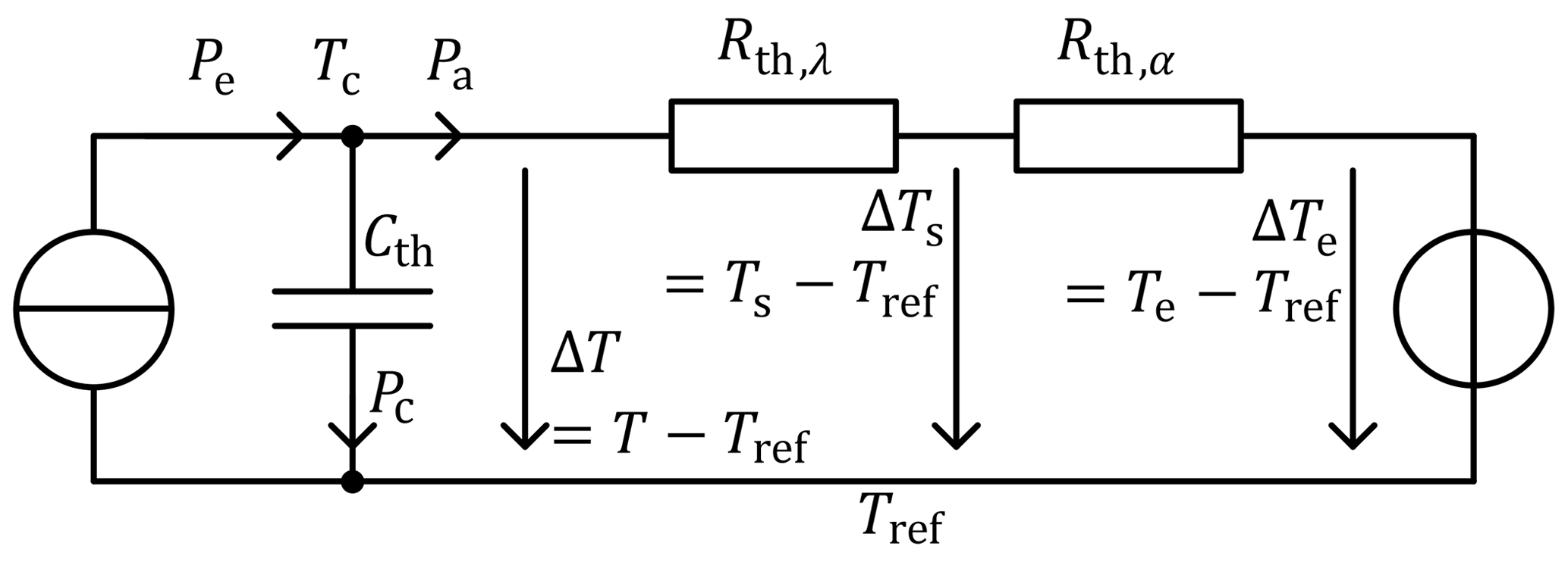
The current I flows through the conductor. The corresponding losses heat up the cable and the heat power P_e is modelled by a heat source. As for typical conductor and insulation materials, the thermal conductance of the insulation is much lower than the conductor's one, the conductor is modelled as an area of constant temperature and the radial heat flow through the conductor is neglected (Wang et al., 2019). The power P_a leaves the system via the surface of the cable. The first law of thermodynamics states

$$\begin{array}{}\text{(9)}& \mathrm{d}{U}_{\mathrm{in}}=\mathit{\delta }Q+\mathit{\delta }W\end{array}$$

where U_in is the inner energy, Q is the heat and W the work. In this case, no work is done at the system, which leads to δW=0. Then, dU_in=δQ follows. The time derivation of this expression leads to

$$\begin{array}{}\text{(10)}& {\displaystyle \frac{\mathrm{d}{U}_{\mathrm{in}}}{\mathrm{d}t}}=\dot{Q}=P_{\mathrm{e}}-P_{\mathrm{a}}.\end{array}$$

Assuming that the inner energy just depends on the temperature, the heat capacitance for a constant volume V and a constant particle number N is inserted:

$$\begin{array}{}\text{(11)}& C_{\mathrm{th}}={\displaystyle \frac{\mathrm{d}{U}_{\mathrm{in}}}{\mathrm{d}T}}\Rightarrow C_{\mathrm{th}}\mathrm{d}T=\mathrm{d}{U}_{\mathrm{in}}\Rightarrow C_{\mathrm{th}}{\displaystyle \frac{\mathrm{d}T}{\mathrm{d}t}}=P_{\mathrm{e}}-P_{\mathrm{a}}.\end{array}$$

This expression behaves as a current through a capacitor. As can be seen, the heat, that is induced in the conductor, splits up into two parts: One part heats up the cable and is therefore stored in the material. The capacitance C_th models this effect. The other part P_a passes the insulation layer (heat conduction, R_th,λ) and leaves the cable at its surface via radiation and convection (R_th,α). The reference potential (temperature) is T_ref. All voltages (temperature differences) refer to this reference. To describe the heat conduction through the insulation layer, Fourier's law is evaluated with the heat conductivity λ of the material:

$$\begin{array}{}\text{(12)}& \begin{array}{rl}{P}_{\mathrm{a}}& =-\mathit{\lambda }A\left(r\right){\displaystyle \frac{\mathrm{d}T}{\mathrm{d}r}}=-\mathit{\lambda }\cdot \mathrm{2}\mathit{\pi }rL\cdot {\displaystyle \frac{\mathrm{d}T}{\mathrm{d}r}}\\ & \Rightarrow T\left(r_{\mathrm{1}}\right)-T\left(r_{\mathrm{2}}\right)=\underset{r_{\mathrm{1}}}{\overset{r_{\mathrm{2}}}{\int }}{\displaystyle \frac{P_{\mathrm{a}}}{\mathrm{2}\mathit{\pi }rL\mathit{\lambda }}}\mathrm{d}r={\displaystyle \frac{P_{\mathrm{a}}}{\mathrm{2}\mathit{\pi }L\mathit{\lambda }}}\ln \left({\displaystyle \frac{r_{\mathrm{2}}}{r_{\mathrm{1}}}}\right)\\ & \iff T_{\mathrm{c}}-T_{\mathrm{s}}=P_{\mathrm{a}}\cdot R_{\mathrm{th},\mathit{\lambda }}.\end{array}\end{array}$$

Here, T is the general temperature, whereas T_c is the temperature of the inner conductor and T_s is the conductor surface temperature. Analogously, radiation and convection are described using another thermal resistance:

$$\begin{array}{}\text{(13)}& T_{\mathrm{s}}-T_{\mathrm{e}}=P_{\mathrm{a}}\cdot R_{\mathrm{th},\mathit{\alpha }}.\end{array}$$

The environmental air has the temperature T_e, which is modelled by a temperature source. The reference temperature can still be chosen arbitrarily. For example, the environmental temperature can be used. Then, the temperature source for the environmental temperature is not necessary. Although it might look like heat would flow back into the conductor through the reference potential, this does not happen physically as there is no physically equivalent structure for the reference potential.

So, from the physical effects, directly the corresponding equivalent circuit can be built up. This approach can be transferred to other cable arrangements: for each radial layer, generally, a capacitance and a resistance are used. For typical conductors, the radial thermal resistance can be neglected in comparison to the thermal resistance of insulation layers. Heat sources model the imprinted heat flow and resistances are used to describe the transition to the environment or other cables. Fixed temperatures as for example the environmental temperatures are modelled via ideal temperature sources.

4.3 Comparison between electrical and thermal equivalent circuits

For an infinitesimally short cable segment (length dz), the equivalent circuit presented in Fig. 2 changes to an equivalent circuit with per unit length parameters (see Fig. 3a) just like in the electrical domain. By now, only radial effects were taken into account. The axial heat flow is considered by adding an axial resistance $R_{\mathrm{th}}^{\prime }$ (see Fig. 3b). By changing the temperature source to an equivalent heat source and rearranging the equivalent circuit, Fig. 3c results. The corresponding electrical equivalent circuit is given in Fig. 3d. As can be seen, those two circuits are very similar: By setting the inductance to $L^{\prime }=\mathrm{0}$ and the reference resistance to $R_{\mathrm{0}}^{\prime }=\mathrm{0}$ in the electrical circuit and inserting an extra current source, the thermal circuit is derived from the electrical one. Sources like this one also appear in the electrical domain, if external field excitations exist (Antonini et al., 2013; Paul, 2008). So only very small changes are necessary.

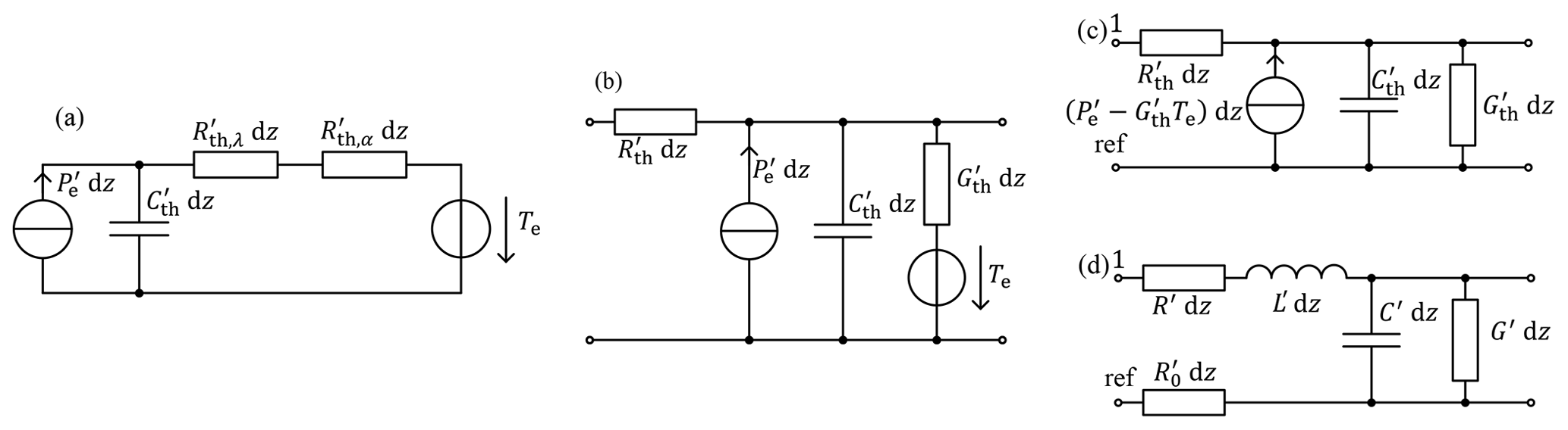
Figure 3 Equivalent circuits for infinitesimally short cable segments of a single cable. (a) Thermal radial model. (b) Thermal axial model. (c) Reduced version of the thermal axial model. (d) Electrical model.

In Fig. 4a, the electrical equivalent circuit for an infinitesimally short segment of (n+1) lines oriented in z-direction is presented (Paul, 2008). One line is chosen as reference conductor. In the thermal domain, the corresponding equivalent circuit for a multiconductor structure can be derived based on the circuit for a single cable. The coupling between the different cables is modelled via additional conductances. In contrast to the electrical domain, capacitive coupling does not appear, as thermal capacitances always refer to the reference temperature. In Fig. 4b, the thermal equivalent circuit is presented. Again, to derive the thermal circuit from the electrical one, only minor changes are necessary as both circuits are very similar to each other. That is why the application of electrical methods to the thermal domain is a promising approach.

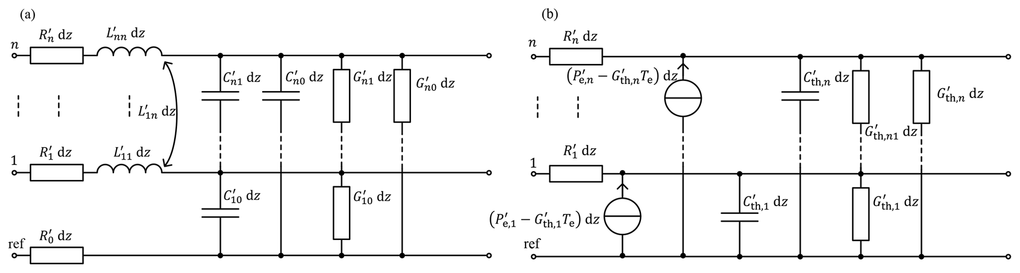
Figure 4 (a) Electrical and (b) thermal equivalent circuit for a multiconductor transmission line segment of infinitesimal length.

In the electrical domain, often, homogenous and lossless environments are assumed. These assumptions cannot be transferred to the thermal domain. That is why some approaches from the electrical domain cannot be used for thermal investigations. Also, in the electrical domain, one conductor is chosen as reference conductor. In the thermal domain, there is no physical reference conductor. That is why in the electrical domain, kind of one additional degree of freedom exists for symmetrical configurations. Nevertheless, as shown before, the equivalent circuits in both domains are very similar, which enables the usage of methods from the electrical domain for thermal problems.

4.4 Differential equations

From the equivalent circuits, partial differential equations for the conductor temperature T_c and the heat flow P can be derived via Kirchhoff's laws equivalently to the electrical domain. For the single line from Fig. 3c, the coupled problem is formulated as follows:

$$\begin{array}{}\text{(14)}& \begin{array}{rl}& {\displaystyle \frac{\partial }{\partial z}}{T}_{\mathrm{c}}(z,t)=-R_{\mathrm{th}}^{\prime }P(z,t),\\ & {\displaystyle \frac{\partial }{\partial z}}P(z,t)=-C_{\mathrm{th}}^{\prime }{\displaystyle \frac{\partial }{\partial t}}{T}_{\mathrm{c}}(z,t)-P_{\mathrm{e}}^{\prime }-G_{\mathrm{th}}^{\prime }\left(T_{\mathrm{c}}(z,t)-T_{\mathrm{e}}\right).\end{array}\end{array}$$

Those equations are quite similar to the corresponding electrical equations. Substituting one equation into the other leads to the parabolic partial differential equation just for the temperature:

$$\begin{array}{}\text{(15)}& \begin{array}{rl}{\displaystyle \frac{\mathrm{1}}{R_{\mathrm{th}}^{\prime }}}{\displaystyle \frac{{\partial }^{\mathrm{2}}}{\partial z^{\mathrm{2}}}}{T}_{\mathrm{c}}(z,t)& -C_{\mathrm{th}}^{\prime }{\displaystyle \frac{\partial }{\partial t}}{T}_{\mathrm{c}}(z,t)-G_{\mathrm{th}}^{\prime }{T}_{\mathrm{c}}(z,t)\\ & =P_{\mathrm{e}}^{\prime }-G_{\mathrm{th}}^{\prime }{T}_{\mathrm{e}}.\end{array}\end{array}$$

If not only a single cable, but a multiconductor structure appears as presented in Fig. 4, the scalar expressions need to be extended to matrix-vector-expressions as in the electrical domain:

$$\begin{array}{}\text{(16)}& \begin{array}{rl}& {\displaystyle \frac{\partial }{\partial z}}{\mathit{T}}_{\mathrm{c}}(z,t)=-{\mathbf{R}}_{\mathrm{th}}^{\prime }\mathit{P}(z,t),\\ & {\displaystyle \frac{\partial }{\partial z}}\mathit{P}(z,t)=-{\mathbf{C}}_{\mathrm{th}}^{\prime }{\displaystyle \frac{\partial }{\partial t}}{\mathit{T}}_{\mathrm{c}}(z,t)-{\mathit{P}}_{\mathrm{e}}^{\prime }-{\mathbf{G}}_{\mathrm{th}}^{\prime }\left({\mathit{T}}_{\mathrm{c}}(z,t)-{\mathit{T}}_{\mathrm{e}}\right).\end{array}\end{array}$$

The corresponding system just for the conductor temperatures is

$$\begin{array}{}\text{(17)}& \begin{array}{rl}{\displaystyle \frac{{\partial }^{\mathrm{2}}}{\partial z^{\mathrm{2}}}}{\mathit{T}}_{\mathrm{c}}(z,t)& -{\mathbf{R}}_{\mathrm{th}}^{\prime }{\mathbf{C}}_{\mathrm{th}}^{\prime }{\displaystyle \frac{\partial }{\partial t}}{\mathit{T}}_{\mathrm{c}}(z,t)-{\mathbf{R}}_{\mathrm{th}}^{\prime }{\mathbf{G}}_{\mathrm{th}}^{\prime }{\mathit{T}}_{\mathrm{c}}(z,t)\\ & ={\mathbf{R}}_{\mathrm{th}}^{\prime }\left({\mathit{P}}_{\mathrm{e}}^{\prime }-{\mathbf{G}}_{\mathrm{th}}^{\prime }{\mathit{T}}_{\mathrm{e}}\right).\end{array}\end{array}$$

Comparing this expression with the corresponding expression in the electrical domain, see Eq. (2), shows the following differences. In the electrical domain, hyperbolic equations describe an oscillating system. The second time derivative corresponds to an oscillating behavior, the first time derivative describes an attenuation. Unlike, in the thermal domain, there is no inductance equivalent. Therefore, wave phenomena as reflections, standing waves and resonances do not appear in the thermal domain.

As there is no capacitive coupling between the different conductors, the matrix ${\mathbf{C}}_{\mathrm{th}}^{\prime }$ is diagonal. Contrarily, in general, in the corresponding electrical matrix C^′, also non-diagonal elements appear. Therefore, the thermal matrix is less complicated than the electrical one in this case and can be regarded as simpler special case of the electrical general case.

5 Application example and first results

In this chapter, exemplary methods for thermal temperature calculation based on the electrical TL theory are summed up and some results are given. The calculation results are compared to the numerical temperature distribution calculated with the FEM software COMSOL Multiphysics (COMSOL Multiphysics, 2021) for the axial temperature distribution and measurement data for the transient temperature development for a long cable.

5.1 Exemplary methods for temperature calculation based on electrical methods

In this section, two approaches for the temperature calculation are shortly presented. Both of them are based on methods known from the electrical domain.

5.1.1 Analytical solutions of the differential equation

The differential equation for a single cable can be solved analytically. This approach was earlier presented in Henke and Frei (2020). If only the stationary axial solution should be calculated, the time dependency and therefore also the time derivative vanishes, and the solution of the differential equation can directly be calculated in the time domain. Also, for the transient radial solution, the axial heat flow is neglected and therefore, the z-derivative vanishes. The reduced differential equation can be solved in the time domain. When both, axial and transient temperature developments have to be considered, the Laplace transform can be used to find a solution for special conditions as a constant current through the cable that is switched on at the beginning of the observation time, a constant cable temperature at the beginning and constant cable end temperatures. The partial differential equation with the boundary conditions is transformed into the Laplace domain. There, a solution is found. Nevertheless, the expression cannot be transformed back into the time domain analytically. That is why an approximation is necessary that enables an analytical transformation (Henke and Frei, 2020). In the thermal domain, the heat source $P_{\mathrm{e}}^{\prime }$ depends on the conductor temperature of the cable and the parameter $G_{\mathrm{th}}^{\prime }$ depends on its surface temperature. That is why a self-consistent nonlinear problem needs to be solved here. An iterative approach that converges very fast is proposed to include those dependencies in Henke and Frei (2020).

5.1.2 Cascading of equivalent circuits

In the electrical domain, equivalent circuits for short cable segments can be cascaded to model the axial development. This approach can equivalently be used in the thermal domain. At the cable ends, sources are used to model a fixed temperature. As for example presented in Önal and Frei (2018), the resulting complete equivalent circuit is implemented and solved numerically in MATLAB/Simscape.

5.2 Axial temperature distribution

In this chapter, for an exemplary setup, the two methods presented above are validated with the FEM software COMSOL Multiphysics (COMSOL Multiphysics, 2021). Here, just a single conductor cable is evaluated, so the problem is rotationally symmetrical. That is why only a two-dimensional discretization is necessary in COMSOL.

A PVC-insulated 2.5 mm² copper cable with the length 0.7 m has the temperature 25 ^∘C at the time t=0 s. At this point, a current of 40 A is switched on. It is assumed that the one end of the cable is connected to the ambient temperature of 25 ^∘C, whereas the other end is connected to a warmer region and therefore has the temperature 85 ^∘C. For this setup, the axial temperature distribution along the cable is calculated for the three points in time t₁=50 s, t₂=200 s and t₃=1000 s. The calculation results are presented in Fig. 5. As can be seen, both, the analytical solution and the Simscape implementation of the equivalent circuit generally fit well with the COMSOL solution. In the transient area (t₁ and t₂), deviations up to 2.5 K appear between the analytical solution and the solutions from COMSOL and Simscape. For the stationary case, all three solutions are close to each other especially in the middle of the cable. The boundary conditions are fulfilled for both solutions very precisely (deviation lower than 0.001 K). Generally, the proposed approaches are able to model the transient axial temperature distribution with a high accuracy, so the approximation in the analytical solution does not cause relevant deviations in this application case.

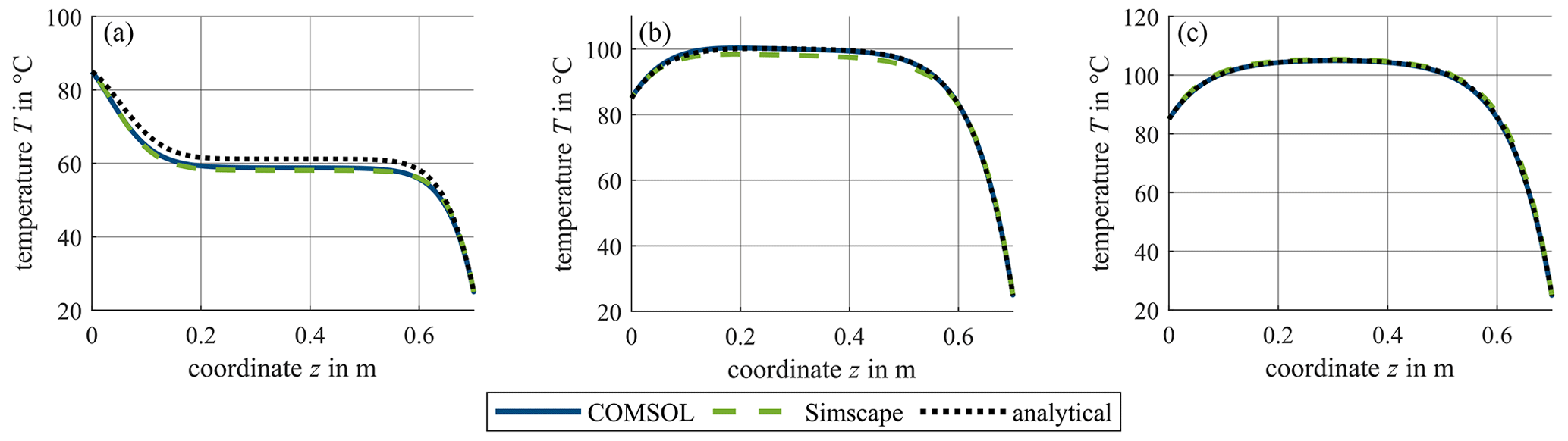
Figure 5 Temperature calculation results along the cable for the times (a) t₁=50 s, (b) t₂=200 s and (c) t₃=1000 s.

5.3 Transient temperature development

In the next step, the transient temperature development for a long PVC insulated 2.5 mm²-copper cable is measured in the middle of the cable via measuring the cable resistance. In this case, the environmental temperature is 21.3 ^∘C. The results are used to validate both of the above presented approaches. At the beginning of the measurement, a current of 25 A is switched on. After 400 s, the current is increased to 35 A. The measurement results are compared to the calculated temperatures using the analytical solution and the Simscape implementation (see Fig. 6). During the first time interval between 0 and 400 s, where the current is 25 A, the measured and calculated temperature are close together. At the end of the interval, a temperature of 50 ^∘C is reached. In the second time interval between 400 and 900 s, the calculated temperatures for the stationary case (end of the interval) are a little higher than the measured temperatures (less than 3 K deviation). As both calculated solutions are very close to each other it can be assumed that parasitic effects that were not modelled in the basic equivalent circuit influenced the measurement results. Nevertheless, the good accordance shows that the presented approaches based on the electrical TL theory can be used to model the real physical behavior of the cable.

Figure 6 Comparison between measurement and temperature calculation results in the middle of the cable along time.

6 Summary

In this contribution, the potentials of applying methods from the electrical TL theory to thermal problems were discussed. Those two domains were compared, and essential physical backgrounds were presented. For two exemplary methods from the electrical domain, it was shown that they are applicable to thermal problems as well. In further research, detailed discussions for additional methods and more complex application examples including the potentials and limits of their applicability in the thermal domain need to be performed.