 | 17 Dec 2021
Simulation of GPS localisation based on ray tracing
Björn Friebel
Michael Schweins
Nils Dreyer
In recent years, many simulation tools emerged to model the communication of connected vehicles. Thereby, the focus was put on channel modelling, applications or protocols while the localisation due to satellite navigation systems was treated as perfect. The effect of inaccurate positioning, however, was neglected so far. This paper presents an approach to extend an existing simulation framework for radio networks to estimate the localisation accuracy by navigation systems like GPS, GLONASS or Galileo. Therefore the error due multipath components is calculated by ray optical path loss predictions (ray tracing) considering 3D building data together with a well-established model for the ionospheric error.
- Article
(2172 KB) - Full-text XML
- BibTeX
- EndNote


When modelling the communication of connected vehicles, most simulation tools assume a precise positioning of transmitter (TX) and receiver (RX). A vehicle's position is the basis of the decision-making process whether sending a message or not. The localisation of a vehicle is mainly based on Global Navigation Satellite Systems (GNSS), because they are widely available on the earth surface. But GNSS-systems are based on several assumptions to work correctly. Therefore simulating the effect of the GNSS-System on localisation is prerequisite for further simulations of connected vehicles.
For a 3D localization, the signal of at least four satellites must be decodable, each enabling to estimate the distance between the receiver (RX) and the satellite (TX). To determine the distance, the receiver assumes the signal to propagate along the direct path and to travel at constant speed of light. However, due to the long distance between the TX and RX, signal propagation is affected by external effects. Especially in urban environments, a direct path is not always guaranteed. Ray optical path loss predictions enable to model the propagation by determining the true geometric distance between the TX and RX. Furthermore, considering all valid paths from the satellite to the device yields the channel gain, making it possible to compute the corresponding received power. Multipath modelling for GNSS using a ray tracing approach is already presented in Lau and Cross (2007) for Carrier-Phase Observations. Another approach for modelling the multipath effect on GNSS is introduced by Wen et al. (2018) using a 3D LiDAR and building height data. Both publications focus on how to eliminate the effect of multipath on GNSS systems. In Jacob et al. (2009) a ray tracing based deterministic simulation model is used to perform the GPS outdoor-to-indoor channel simulations. Neuland et al. (2011) investigated the influence of the GPS-based positioning on deriving radio maps for self-organizing networks (SON) using software simulation.
In addition, as specific nature of satellite-to-earth links, that signal has to pass the atmosphere of the earth. As a consequence the different layers of the atmosphere like troposphere and ionosphere have to be considered in modelling propagation as well. The ionosphere is a dispersive medium resulting in a frequency-related slowing-down effect on the signal depending on the geometry between the TX and RX and the time-variant state of the sun. In contrast, the troposphere is a non-dispersive medium and according to the ITU Recommendation ITU-P.531-13 (ITU, 2016) the effect of the troposphere is negligible compared to the effect of the ionosphere. Modelling the effect of the ionosphere is mentioned in several publications (e.g., Alizadeh et al., 2015).
In contrast to all these publications, this research focus not only on multipath or ionosphere modelling, but to combine both and integrate it into an existing simulation tool with a focus on localisation accuracy. Furthermore this paper demonstrates how to extend this simulation tool usually used for mobile networks on earth with the ability to propagate satellite-to-earth links.
Models for multipath propagation and the ionosphere were integrated in the Simulator for Mobile Networks (SiMoNe) framework developed at the Institute for Communications Technology, Braunschweig, making it possible to evaluate positions along a trace with different focal points: on the one hand, visible and receivable satellites were evaluated to identify dead spots. On the other hand, determining localisation accuracies can lead to conclusions about areas with a high probability of insufficient positioning.
This paper is structured as follows: A guide for preparing the simulation data is proposed in Sect. 2. Afterwards, Sect. 3 presents a concept of ray-optical pathloss predictions for GNSS radio links (Sect. 3.1) together with a model for the ionosphere (Sect. 3.2). In Sect. 4 the results of ray tracing and ionosphere propagation are used for determining the localisation accuracy and for computing the positioning error. The methods proposed in this paper are validated by a measurement in Sect. 5. Results from this measurement (Sect. 6) and a subsequently discussion (Sect. 7) are concluding this paper.
To simulate satellites by using ray optical pathloss predictions a valid scenario is required. Information about buildings in 3D can be modelled based on open street maps (OpenStreetMap Foundation, 2021). Antenna patterns for L1/L1C frequencies are open to the public on a US-government-hosted website about GPS (USCG, 2021). The number of sun spots for a particular month, used for modelling the ionosphere can be extracted from space weather websites (e.g., SpaceWeatherLive, 2021).
Satellite positions are described by their orbit and a timestamp. Any GPS-Receiver receives these information via the GPS-Signal. For our simulations we use publicly available orbit data, the almanach (Kelso, 2021). The calculation of satellite positions based on orbit data can be found in GPS-Standardisations (GPS-SEI, 2019, 20-IV). As a result the satellite positions are given in geocentric coordinates, called Earth-Centered-Earth-Fixed (ECEF).
For use in simulation, geocentric coordinates have to be harmonized with geodetic coordinates of buildings and subscriber positions. Usually, buildings and subscriber positions are in a projected coordinate system based on an assumption of the earth shape like the Universal Transversal Mercator (UTM) or Gauß-Krüger (GK) system. The ray tracer used for this paper is based on cartesian coordinates and can not work with angular coordinate systems, like the World-Geodetic System 84 (WGS84). As a consequence there are two options to choose from: Transform buildings and subscriber cordinates into ECEF or transform the satellite positions into UTM/GK.
Using a common projection algorithm to project WGS84 coordinates into UTM/GK leads to distortions up to 40 cm/km starting at meridian. Therefore following solution is used: First, a position on earth ground is defined as reference. This reference position is transformed from UTM/GK to WGS84 and converted to ECEF coordinates. Secondly, the reference position is defined as origin of its local coordinate system in a Earth-North-Up (ENU) orientation. The relationship between a global ECEF- and a local ENU coordinate system is shown in Fig. 1. The local ENU coordinate system spans a tangential plane to the earth surface in x- and y-direction. The z-axis is orthogonal to the earth surface in a upwards direction. A closed-form algorithm by Vermeille (2011) is used for the transformation from geocentric (ECEF) to geodetic (WGS84) coordinates. Finally, all satellites are also converted into the predefined local coordinate system of the reference position. The local satellite coordinates are used for determining the position in UTM/GK by adding it to the reference position in projected coordinates.
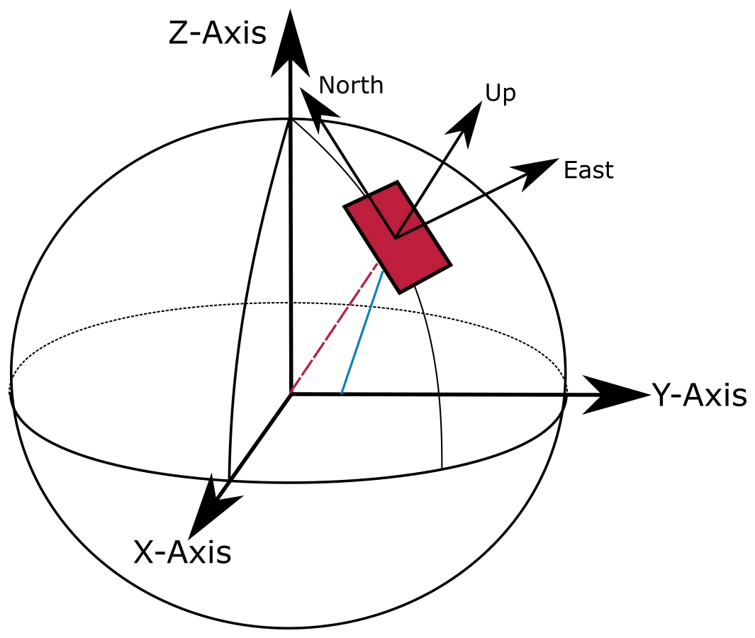
Figure 1East North Up (ENU) local coordinate system in relation to Earth Centered Earth Fixed (ECEF) global coordinate system.
As a result the satellite position is a non valid GK/UTM position in the context of using transformation algorithms. But it works under the assumption that most of propagation effects occur near the position on the earth ground. For larger scenarios this solution needs to be repeated for every receiver position to reduce projection distortions.
The section of Propagation Modelling is divided in two parts. The first part is about ray optical propagation predictions in the context of satellites and methods to accelerate checking whether a link exist. The second part is about modelling the ionosphere representing the effect by the atmosphere. From the point of view by ray optical propagation modelling, a ray travelling through the ionosphere is assumed as a straight line. As a consequence, only a slowing effect on the propagation is modelled.
3.1 Channel Modelling
The simulation framework for this work is the Simulator for Mobile Networks (SiMoNe), developed at the Institute for Communications Technology at TU Braunschweig (Rose et al., 2015). Initially, SiMoNe was developed as simulator for radio network planning on system-level. Now SiMoNe supports different channel models including 3D ray optical propagation enabling link-level simulations. New fields of application for SiMoNe are device to device use-cases in the context of V2V (Dreyer and Kürner, 2019) and Terahertz Communication (Kürner et al., 2020).
In contrast to these use cases, a satellite to earth link differ from mobile communication in the field of distance and propagation effects. GPS-Satellites travel on a height of 20 200 km above the earth ground, which defines the minimum signal path length. As mentioned in Sect. 2, obstacles blocking the signal path (here buildings) have to match the coordinate system of the transmitter and receiver. In radio networks the distance between TX and RX is significantly lower (several km). Beside the effect of a greater distance, elevation angles differ from base station to receiver constellations: Satellites appear in all possible elevation angles. Also satellites can be almost parallel to the earth ground and disappear for a certain time below the horizon.
A link budget, including transmission power, attenuation by multipath components and antenna masking, is an enabler to identify visible and decodable satellites of the specific user. Also the path of the channel components can be used for modelling the error by multipath. GNSS-Receiver can use two techniques to estimate the signal duration: Code-Phase (CoP) or Carrier-Phase (CaP) observation. CoP observation uses the coded signal for correlation and CaP observation uses the original modulated signal. The technique of observing the CoP is not as distinct as the CaP and can lead to errors of tenth of meters due to multipath error (Betz, 2015, p. 144). Nevertheless, using the CoP technique a position is faster evaluated than in a CaP observation. In this work, we used following equations from Liso and Kürner (2014) to determine the multipath error in meter.
For Carrier-Phase Observation Eq. (1) is used. The first factor transforms the bias from radians to meter with λ being the wavelength. The mth ray stands for the most powerful ray related to the channel gain. Under LOS condition, ΔϕNLOS=0, whereas under NLOS condition , where θm is the phase of the most powerful ray and Φ is the true distance between satellite and receiver. N is the total number of rays. All terms in the sum are calculated with respect to the most powerful ray, so that with Am being the amplitude of the most powerful ray, and Ai the amplitude of the ith ray. Δθi=θi−θm is the phase difference between the most powerful ray and the ith ray.
For calculating the multipath error for Code-Phase Observation ΔΦ Eq. (2) is used.
l stands for the path length. ΔlNLOS=0 in case of LOS, ΔlNLOS=lm−Φ under NLOS, and Δli=li−lm is the path length difference between the most powerful ray and the ith ray.
The variables mentioned in both equations can be derived from the results of ray tracing.
Acceleration options for Satellite-Earth Links
Before starting ray optical path loss predictions, determining which satellites are visible in the context of a receiver position reduces overhead. Therefore each elevation angle between the receiver and satellite position needs to be calculated. An positive elevation angle represents a visible satellite above the horizon.
Instead of calculating elevation angles and transforming all coordinates of the buildings for each receiver position, an assumption can be made. If the scenario is assumed to be small in comparison to the distance between satellite and ground level and in comparison to the appearing projection errors, we can use one receiver position as a reference position for the whole scenario. Usually the centre point of all buildings in the scenario is chosen as a reference position.
A common speed up algorithm to filter buildings of interest for ray tracing is using an ellipse with TX and RX in the focal points and a configurable extra path length. This filter is not usable here. Since the great distance in combination with a wide variety of elevation angles leads to a ellipse either excluding or including all buildings. The ellipse approach functions well, if obstacles are equally distributed between the transmitter and receiver. But any possible obstacle obstructing the signal path in satellite to earth links is located next to the receiver. Therefore an obstacle filter should concentrate on the receiver position. A rectangle or a circle around the receiver position are feasible forms for filtering.
3.2 Ionosphere
The ionosphere is a dispersive medium. As mentioned before, the ionosphere has a negligible effect on the path geometry but on the velocity of the electromagnetic wave. The slowing-down effect depends on the number of electrons in the ionosphere layer which can be described by the Total Electron Count (TEC). The sun activity is responsible for ionizing the atmospheric layer. So the number of electrons are depending on the sun activity. An indicator for the sun activity is the number of sun spots. The more sun spots exists, the higher is the electron density in the ionosphere. Sun spots are described within a sun cycle which changes over several years. Another factor related to the sun is the time of day. By night the effect of the sun is less present than during the day. Therefore the ionospheric effect is related to the simulation time and need to be modelled by the sun spot number and time of day.
Based on ITU-P.531-13 (ITU, 2016) two approaches modelling the ionosphere are proposed: International Reference Ionosphere (IRI-2012) and NeQuick2. We decided to use the NeQuick2 model, because of the limited range of 2000 km in the IRI-2012 model.
NeQuick2 models the Slant Total Electron Count (STEC), same as the TEC along a ray path (Nava et al., 2008). The tool is written in the programming language Fortran77 and needs the sun spot number, the point of time and date, and the positions of TX and RX in a spherical coordinate system as input.
Following Eq. (3) by Zolesi and Cander (2014, p. 78) calculates the delay in meter df based on STEC, frequency f and a constant factor K=40.3.
NeQuick2 was fully integrated in SiMoNe.
Pseudoranges describe the distance between satellite and receiver based on measuring the signal delay by the receiver, which includes all errors. As a consequence in the simulation the errors by multipath propagation and ionosphere delay have to be added to the true distance. Calculating the pseudorange is carried out only for visible and receivable satellites based on ray-optical predictions.
For a 3D position a receiver needs at least four visible and decodable satellites available. The process of determining a position based on pseudoranges is called multilateration.
Multilateration describes the algorithm of finding the intersection of all spheres with the radius of the pseudoranges. The relations between pseudoranges and the searched position for each satellite i can be written in an equation system, as follows:
On the left hand side of the equation system is the pseudorange as a product of pseudodelay Di and speed of light c0. Pseudodelay Di describes the signal propagation time measured at a receiver assuming only a direct signal path between satellite and receiver. On the right hand side are the differences between coordinates of the satellite () and the sought position (). Furthermore a delay of c0⋅Δt is added representing the clock offset Δt between receiver and transmitter.
At least four satellites are needed to determine the four variables in this equation system. There exist several algorithms to solve this equation system by an iterative approach or in a closed-form algorithm. For our simulations a closed-form algorithm, called the Bancroft-Algorithm (Bancroft, 1985), is used. To solve these equations the Bancroft algorithm changes the pseudoranges by the same factor to find the intersection of all spheres with the radius of the modified pseudoranges.
If the receiver can decode more than four satellites, the equation system is overdetermined. There are two options to handle this: on the one hand the receiver can choose four satellites based on the constellation geometry and exclude all other satellites. On the other hand all visible and decodable satellites are integrated and used for determining a position. Both options were implemented.
Localisation accuracy
To assess the accuracy of a satellite-based localisation system, at least three indicators exists: The Dilution of Precision (DOP), comparing a simulated absolute position with a true position, and a deviation range within the true position shall exist with a given probability.
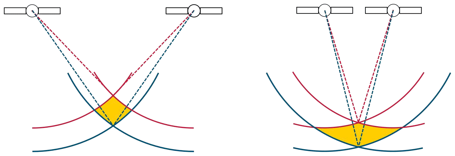
The constellation of the satellites can be described by DOP. DOP is an qualitative measure to evaluate the constellation quality by the volume of the satellites span. In Fig. 2 two different satellite constellations are shown. Two potential pseudoranges are drawn for each satellite. The true position is located within the area between the pseudorange's circles. On the left-hand side the constellation of satellites is more advantageous than the satellite constellation on the right-hand side, because of a smaller area in which the true position could be located. Therefore, having satellites distributed in different directions and with a proper distance to each other, the error probability is reduced.
With the help of multilateration algorithm, an absolut position can be determined. The effect of the error sources are represented in the difference between the calculated and the true position and gives a statement about the localisation accuracy.
An alternative to an absolute positional difference for evaluating localisation accuracy is using an statistical measure like CE90. CE90 indicates a radius of circle that covers the RX position by a chance of 90 %. The Eq. (5) for calculating a CE90 value is given and defined in Betz (2015, p. 149).
CE90 is based on the DOP value, here in the horizontal layer (HDOP) and the User Equivalent Range Error (UERE). The UERE, also called pseudorange-error, contains all errors from the state of generating the GNSS-Signal up to the state of receiving the signal. Errors based on multipath propagation and the ionosphere are included in the UERE.
For evaluation of the proposed methods a measurement was made. The first method to prove is the coordinate transformations described in Sect. 2. If the same satellites are visible, azimuth and elevation angles match, and the constellation quality based on DOP values fit with the measurement. The results produced by ray tracing like the received power should match the measurements and the same satellites should be decodable. The ionospheric error is calculated by NeQuick2 (Sect. 3.2) and the TEC values should match daily updated maps published by space weather providers.
5.1 Measurement
The core at the measurement setup is a application board with a ZED-F9P module by u-blox functioning as a GNSS-Receiver. It allows to record and export GPS-Logs in a NMEA-Format. From these messages, the date, time, position in degrees minutes, DOP Values, elevation and azimuth angles and CNDR can be extracted. CNDR stands for Carrier-to-Noise-Density-Ratio, expressed in dBHz and is often used in the context of satellite communications.
The receiver is capable of combining information from different satellite localisation systems like GPS, GLONASS, and Galileo. It can also be used as a dual frequency receiver and works with additional correction information from earth stations. Any feature going beyond a single-frequency-receiver without correctional parameters is turned off to reduce uncertainties in comparison with the simulation.
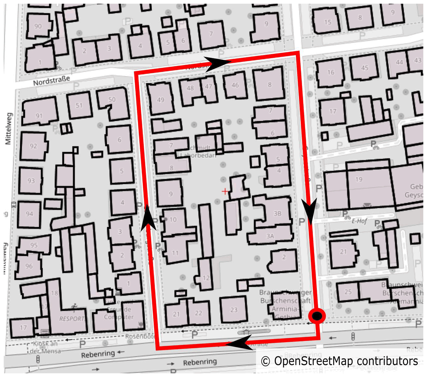
Figure 3Map of Braunschweig (Germany) including modelled buildings and route of measurement based on © OpenStreetMap contributors 2021. Distributed under the Open Data Commons Open Database License (ODbL) v1.0.
The measurement was performed in northern Braunschweig at 09:15:00 UTC on 12 January 2021. In Fig. 3 the map section and the route of the scenario is drawn. Start and end position of the route is marked as a circle. We drove the route by car in clock-wise direction with the GNSS-Antenna on top of the car roof.
5.2 Simulation
First the choosen configuration for transmiter and receiver in the simulation will be explained. It is assumed that the satellites transmit with a power of 47 dBm (Betz, 2015, p. 107). The antenna diagrams for satellites published by USCG (2021) are used to determine the transmitter antenna gain as a function of satellite orientation and elevation angle. The antenna diagram for the receiver is unknown and the antenna gain is set to 0 dBi. u-blox, producer of the GNSS-Receiver used in the measurement, states a receiver sensitivity of −157 dBm for tracking and navigation.
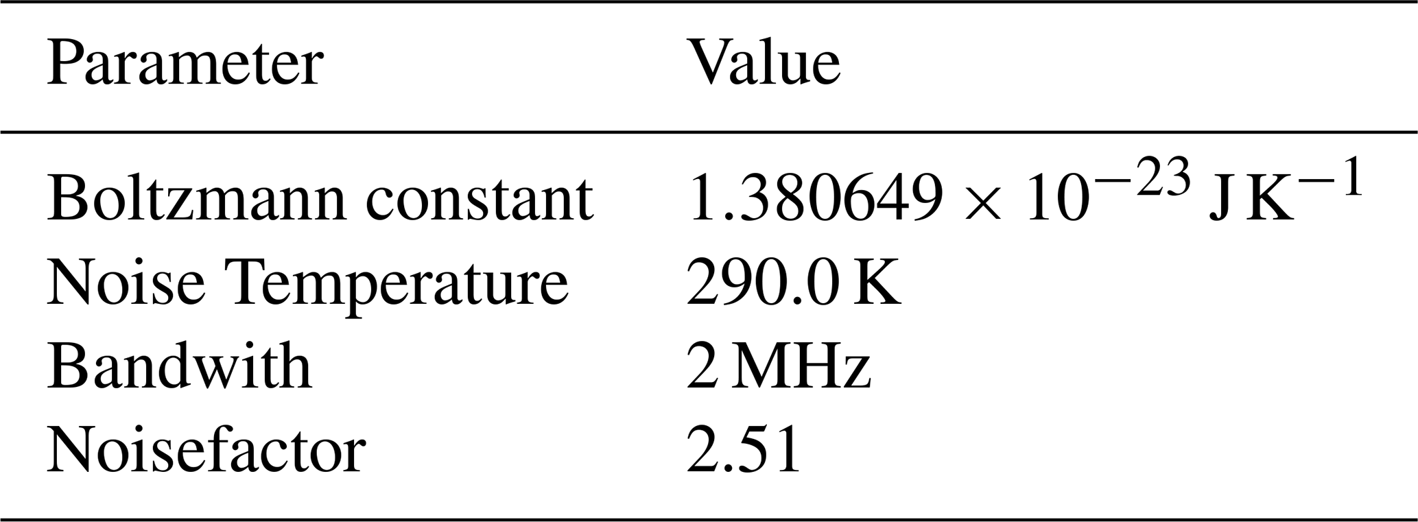
In the GPS-Logs the power is given as Carrier-to-Noise-Density-Ratio (CNDR). System parameters to calculate the CNDR based on a received power are presented in Table 1.
In the following the configuration of the ray tracer is presented. Most common frequency band used for GPS is the L1/L1C frequency. Therefore the frequency is set to 1575.42 MHz. Corresponding material parameters for frequencies above 100 MHz are available in ITU (2015). Beside a direct path, the ray tracer is configured to find reflections up to an order of two and diffractions on building roofs. To accelerate the ray tracing, the algorithm presented in Sect. “Acceleration options for Satellite-Earth Links” with a square width of 100 m for the bounding box is used. In the time period of the measurement the number of sun spots is zero.
A satellite constellation diagram is shown exemplary for one timestep in Fig. 4. The maximum deviation of the elevation angle between simulation and measurement is 0.47∘ and for azimuth angle 0.31∘. The same GPS-Satellites are visible in simulation and measurement.
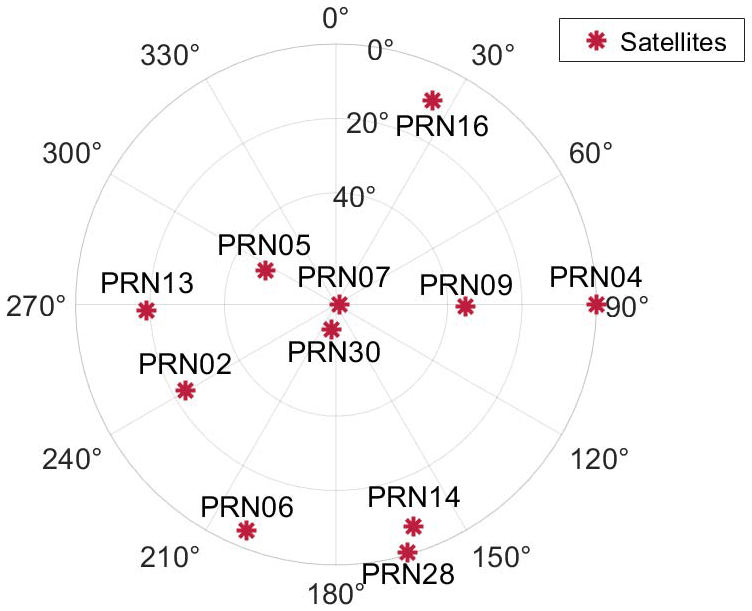
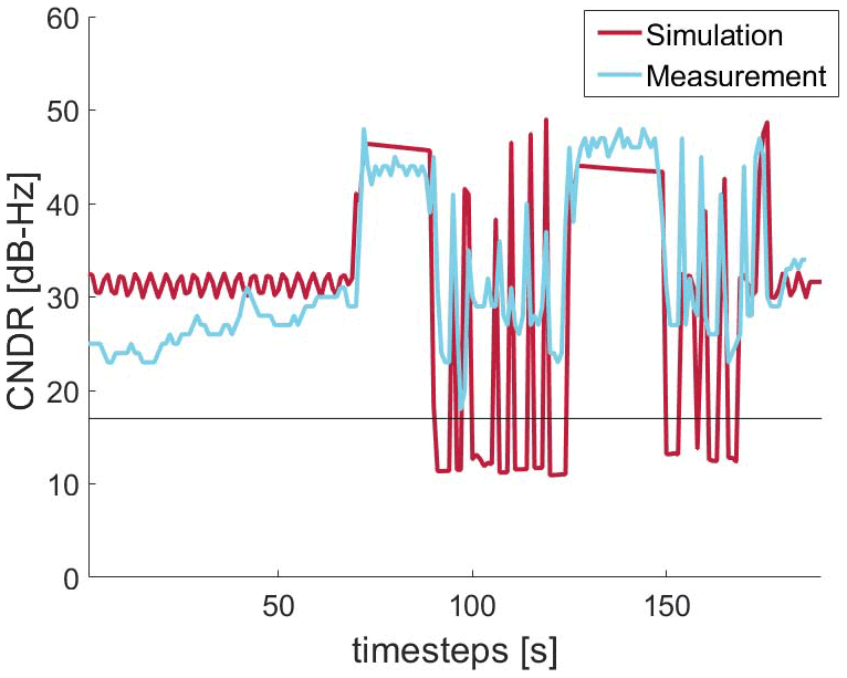
Figure 5CNDR for satellite PRN13 from 09:15:00 to 09:18:10 UTC on 12 January 2021 along a measured path.
Figure 5 shows for the GPS-satellite PRN13 the CNDR in dBHz in comparison between simulation and measurement. The receiver sensitivity of −157 dBm (17 dBHz) is drawn as threshold for a decodable satellite. Satellite PRN13 is located to the west of the scenario and on an elevation angle of 20∘. Therefore we expect in this scenario Line-Of-Sight (LOS) links in street canyons parallel to the satellite-receiver-link and mostly Non-Line-Of-Sight (NLOS) links in street canyons orthogonal to the satellite-receiver-link. The intervals from 70 to 90 s and from 125 to 147 s are dominated by LOS-links with CNDR values between 40 and 50 dBHz. These periods can be identified as the street canyons parallel to the satellite-receiver link. Measurement and simulation differ by 4 to 5 dB. In street canyons orthogonal to the satellite to receiver link NLOS links are mostly present, interrupted by LOS links resulting from gaps between the buildings. If the ray tracer only finds a diffracted ray on the roof, the resulting power is less than the receiver sensitivity. In contrast to that, the measurement produces values above the receiver threshold. As a result satellite PRN13 is not counted as decodable in these time intervals.

Figure 6Position deviation between Simulation (Carrier-Phase) and Measurement from 09:16:10 to 09:18:00 UTC on 12 January 2021 along a measured path
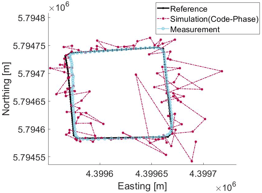
Figure 7Position deviation between Simulation (Code-Phase) and Measurement from 09:16:10 to 09:18:00 UTC on 12 January 2021 along a measured path
In Figs. 6 and 7, the result of using the Bancroft-Algorithm (Sect. 4) for Carrier-Phase (CaP) and Code-Phase (CoP) observation in addition to the ionosphere error is shown. Also the ideal trace and the measured path are drawn in the map. As expected the error in multipath by CoP observation results is higher than those of CaP observation, which results in position deviations more than a few meters. The positions calculated on base of CaP observations match the ideal trace positions almost and are closer to the ideal trace than the measured one. The measured trace does not show a higher deviation between the individual positions than expected by the movement of a car. This behaviour results from the effect of the filtering algorithms the receiver uses.
Analysing CE90 values for this measured trace results in similar outcome.
The transformation of coordination results in similar satellite constellations as measured. So the approach of integrating satellites in a non-spheric coordinate, but projected coordinate system, is applicable.
The received power calculated by the ray tracer depends on its configuration with regard of implemented multipath effects, level of detail in modelling obstacles, buildings and receiver equipment. Here the results of LOS links matches the measurement rather good. In the case of NLOS-scenarios there are unmodelled effects, especially in cases with only a diffracted link. Different reasons can lead to this behaviour: first other propagation paths were not modelled, like diffraction on sides of buildings. Secondly, the model of diffraction are not feasible for this scenario. Therefore further development needs to be invested in the ray tracer.
The main problem of comparing the simulation and the measurement is the post-processing made by the GNSS-Receiver. In the simulation, the positions are individual determined. In contrast to that, the positions resulting from the receiver are filtered and CE90 and position offset does not have any information about previous positions, that might be available at the receivers.
In this paper we presented approaches to integrate a simulation model for satellite localisation into an existing simulation framework using ray optical pathloss predictions. As a result we are now able to simulate and do ray-optical analyses of GNSS-Satellites. In the future we extend the ray tracer further to enable multipath options as scattering. Additionally, setting up an own GNSS-Receiver based on Software-Defined-Radios (SDR) allows to extract intermediate states, like pseudoranges to improve and evaluate here proposed methods.
The data presented in this article are available from the authors upon request.
The computer simulations, measurements and results are carried out by BF. Scientific investigations and editorial hints were given by MS and ND. Mentorship including editorial hints were provided by TK.
The authors declare that they have no conflict of interest.
Publisher’s note: Copernicus Publications remains neutral with regard to jurisdictional claims in published maps and institutional affiliations.
This article is part of the special issue “Kleinheubacher Berichte 2020”.
This open-access publication was funded by Technische Universität Braunschweig.
This paper was edited by Madhu Chandra and reviewed by Pierre Reisdorf and Matthias Vodel.
Alizadeh, M. M., Schuh, H., and Schmidt, M.: Ray tracing technique for global 3-D modeling of ionospheric electron density using GNSS measurements, Radio Sci., 50, 539–553, https://doi.org/10.1002/2014RS005466, 2015. a
Bancroft, S.: An Algebraic Solution of the GPS Equations, IEEE T. Aero. Elec. Sys., AES-21, 56–59, https://doi.org/10.1109/TAES.1985.310538, 1985. a
Betz, J. W.: Engineering Satellite-Based Navigation and Timing – Global Navigation Satellite Systems, Signals, and Receivers, John Wiley & Sons, New York, 2015. a, b, c, d
Dreyer, N. and Kürner, T.: An Analytical Raytracer for Efficient D2D Path Loss Predictions, in: 2019 13th European Conference on Antennas and Propagation (EuCAP), Krakow, Poland, 1–5, IEEE, New York City, 2019. a
GPS-SEI: Global Positioning System – Interface Specification (IS-GPS-200K), GPS Directorate Systems Engineering & Integration – LAAFB, U.S. Space Force, The Pentagon, Arlington County, Virginia, 2019. a
ITU: Effects of building materials and structures on radiowave propagation above about 100 MHz (ITU-R Recommendation P.2040-1), International Telecommunications Union, Genf, 2015. a
ITU: Ionospheric propagation data and prediction methods required for the design of satellite services and systems (ITU-R Recommendation P.531-13), International Telecommunications Union, Genf, 2016. a, b
Jacob, M., Schon, S., Weinbach, U., and Kurner, T.: Ray tracing supported precision evaluation for GPS indoor positioning, in: 2009 6th Workshop on Positioning, Navigation and Communication, 2009, 15–22, https://doi.org/10.1109/WPNC.2009.4907798, 2009. a
Kelso, D. T.: GPS SEM Almanacs, available at: https://celestrak.com/GPS/almanac/SEM/, last access: 16 January 2021. a
Kürner, T., Hirata, A., Jung, B. K., Sasaki, E., Jurcik, P., and Kawanishi, T.: Towards Propagation and Channel Models for the Simulation and Planning of 300 GHz Backhaul/Fronthaul Links, in: 2020 XXXIIIrd General Assembly and Scientific Symposium of the International Union of Radio Science, 2020, 1–4, https://doi.org/10.23919/URSIGASS49373.2020.9232186, 2020. a
Lau, L. and Cross, P.: Development and Testing of a New Ray-Tracing Approach to GNSS Carrier-Phase Multipath Modelling, J. Geodesy, 81, 713–732, https://doi.org/10.1007/s00190-007-0139-z, 2007. a
Liso, M. and Kürner, T.: Investigation on the influence of diffraction by wedges in satellite navigation systems, in: The 8th European Conference on Antennas and Propagation (EuCAP 2014), The Hague, the Netherlands, 1598–1602, https://doi.org/10.1109/EuCAP.2014.6902091, IEEE, New York City, 2014. a
Nava, B., Coïsson, P., and Radicella, S.: A new version of the NeQuick ionosphere electron density model, J. Atmos. Sol.-Terr. Phy., 70, 1856–1862, https://doi.org/10.1016/j.jastp.2008.01.015, 2008. a
Neuland, M., Kurner, T., and Amirijoo, M.: Influence of Positioning Error on X-Map Estimation in LTE, in: 2011 IEEE 73rd Vehicular Technology Conference (VTC Spring), Budapest, Hungary, 1–5, https://doi.org/10.1109/VETECS.2011.5956331, IEEE, New York City, 2011. a
OpenStreetMap Foundation: Openstreetmap, available at: https://www.openstreetmap.org/, last access: 16 January 2021. a
Rose, D. M., Baumgarten, J., Hahn, S., and Kurner, T.: SiMoNe – Simulator for Mobile Networks: System-Level Simulations in the Context of Realistic Scenarios, in: 2015 IEEE 81st Vehicular Technology Conference (VTC Spring), Glasgow, UK, 1–7, https://doi.org/10.1109/VTCSpring.2015.7146084, IEEE, New York City, 2015. a
SpaceWeatherLive: Solar Activity, available at: https://www.spaceweatherlive.com/en/solar-activity.html, last access: 16 January 2021. a
USCG: L Band Antenna Panel Patterns And Performance, available at: https://navcen.uscg.gov/?pageName=antennapanels, last access: 16 January 2021. a, b
Vermeille, H.: An analytical method to transform geocentric into geodetic coordinates, J. Geodesy, 85, 105–117, https://doi.org/10.1007/s00190-010-0419-x, 2011. a
Wen, W., Zhang, G., and Hsu, L.-T.: Correcting GNSS NLOS by 3D LiDAR and Building Height, in: 31st International Technical Meeting of The Satellite Division of the Institute of Navigation (ION GNSS+ 2018), 3156–3168, https://doi.org/10.33012/2018.15984, 2018. a
Zolesi, B. and Cander, L. R.: Ionospheric Prediction and Forecasting, Springer-Verlag, Berlin Heidelberg, https://doi.org/10.1007/978-3-642-38430-1, 2014. a