Description of the Coupling of two Loop Antennas using Electrical Equivalent Circuit Diagrams

EMC measurements must be carried out in standardized and defined measuring environments. The frequency range between 9 kHz and 30 MHz is a major challenge for measurement technology. The established test sites are designed with an perfect elelctrically conducting ground. For the considered lower frequency range, the metrological validation is carried out with magnetic field antennas in this frequency range. The aim is therefore to take into account the ferromagnetic properties of the ground plane in such a measurement environment and to describe them analytically or numerically with an electrical equivalent circuit diagram. In this article we simplify the model to two loopantennas in Freespace without groundplane to check if the approache with the ECD will work. Therefore we use various numerical field calculation programs in the frequency range up to 30 MHz. The results from simulations are to be checked for correctness with describing them analytically or numerically. For this purpose, a model consisting of two loop antennas was created and simulated in a numerical simulation program. In order to validate the results from the simulation, two different approaches to creating an electrical equivalent circuit (ECD) are examined. The first approach is based on the real equivalent circuit diagram of a coil and the second approach forms a parallel resonant circuit of the first resonance of an antennas input impedance. The focus here is on the mutual inductance, which represents the coupling between the two antennas.

1 Introduction

EMC measurements of emitted interference and immunity are to be carried out in accordance with CISPR-16 and CISPR-25 in standardized and defined measurement environments like Open Aerea Test Sites (OATS) or Semi Anechoic Chambers (SAC) (IEC/CISPR 16-1-4, 2019). To validate these EMC measuring stations, Trautnitz and Riedelsheimer (2014) carried out a round robin test in different half-absorber chambers and free field measuring stations. The frequency range between 9 kHz and 30 MHz is a major challenge for the measurement technology, as the distance between DUT and the antenna is much smaller than the wavelength of the frequency under consideration. The validation was carried out with magnetic field antennas, as stipulated in the standards for this frequency range. However, the influence of the ground plane in these measuring environments has not been investigated so far. Therefore the aim is to consider the ferromagnetic properties of the ground plane in an SAC or OATS and to describe them analytically or numerically. A first step was an investigation of the influence of a ground plane on the measurement result in the frequency range up to 30 MHz with the aid of various numerical field calculation programs (Rogowski et al., 2018a, b). For the simulation, a simplified arrangement was modeled based on the round robin test mentioned above, which consists of two loop antennas over a ground plane in an otherwise ideal environment.

In this article, the results from the previous simulations are to be checked for correctness. First, a simulation of two loop antenna in the freespace is carried out with a numerical field calculation program based on the method of moments (Concept II) and the feedingpoint voltage is determined. Then the antennas are modeled and calculated in two different ways as an electrical equivalent circuit diagram (ECD) using a circuit simulator (LT-Spice). In the first case, the antenna is modeled as the ECD of a real coil, i.e. lossy with parasitic winding capacitance. This has already been investigated for a single loop antenna, which a plane wave field is applied in a previous work and the comparison of the results from LT-Spice and Concept II shows a good agreement (Rogowski et al., 2020). In the second case, an ECD is modeled that takes into account the first resonance of the input impedance of the antenna. The knowledge gained from this is then used to create a suitable ECD in LT-Spice, which takes into account the two antennas (transmitting and receiving antenna) and their interaction or coupling in the frequency range up to 30 MHz. The focus here is on the mutual inductance between two coils, which represents the coupling between these antennas. The mutual inductance is initially assumed to be a constant. In the next step, in addition to the constant calculated mutual inductance, the influence of the frequency on the magnetic field in the coupling between the antennas should be taken into account.

2 Simulation in freespace

In previous work, the parasitic effects of a loop antenna were investigated in a simulation with a different number of windings and the coupling of the magnetic field into the antenna was implemented with a plane wave field. Loop antennas with one, two and three windings were implemented. In this work, two loop antennas with the same number of wingings as in the previous study are considered in the free space. The focus here is on the coupling of the magnetic field transmitted from the transmitting antenna to the receiving antenna.

2.1 Simulation Model

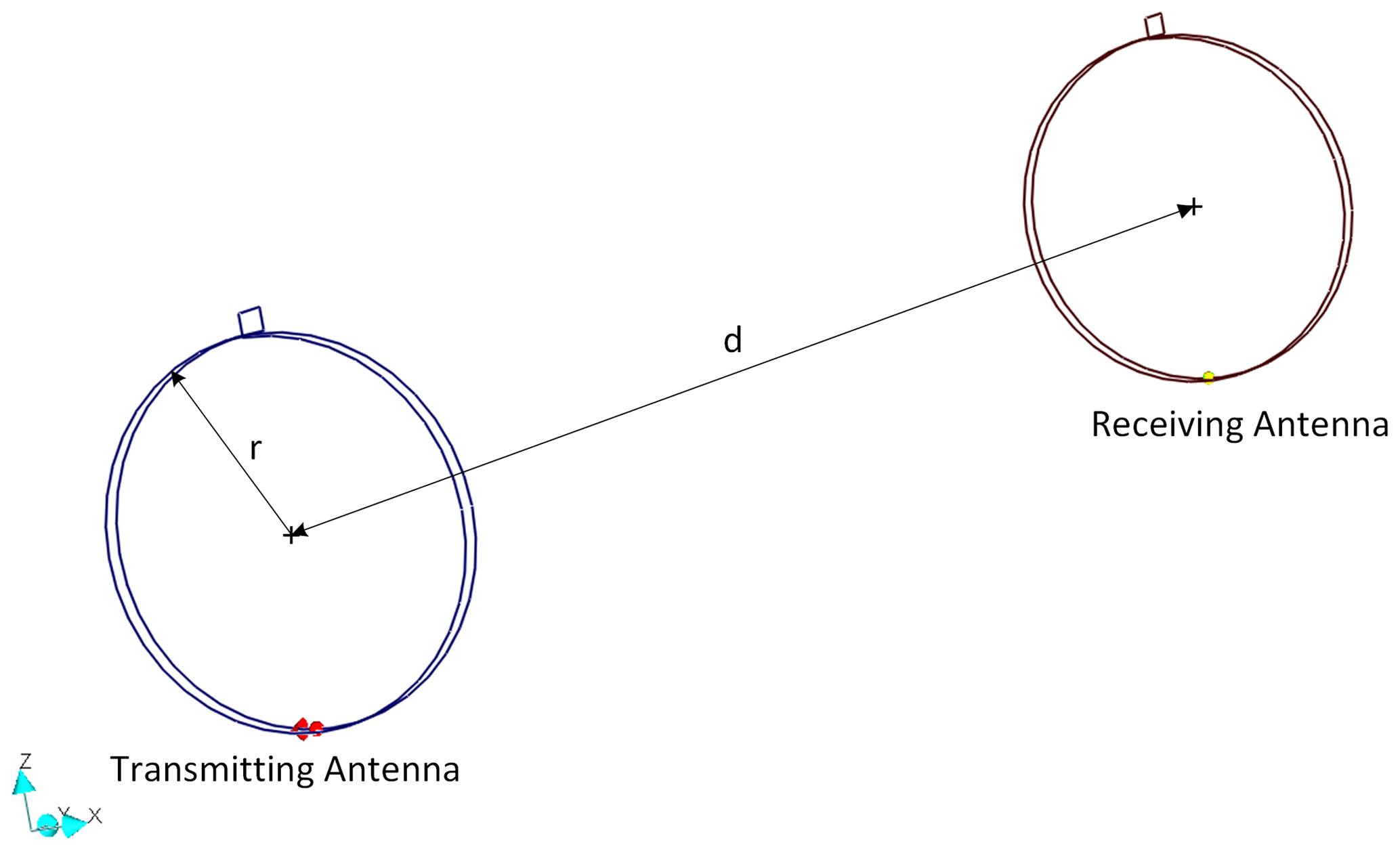
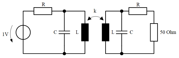
For this purpose, two loop antennas are modeled in a numerical field simulation program (Institute of Electromagnetic Theory, 2018). Both antennas have a radius of 25 cm and are idealized as a round wire. A voltagesource is connected to the transmitting antenna, which feeds 1 V into the antenna. The incoming magnetic field is coupled into the receiving antenna in a distance of 3 m and the feedingpoint voltage of the antenna is determined at a 50 Ω resistor. The two antennas are in coaxial alignment. The frequency range of 9 kHz and 30 MHz is considered. Figure 1 shows the entire simulation model as an example for loop antennas with two windings.

Figure 1 Entire simulation model for two loop antennas with two windings each.

2.2 Simulation Results

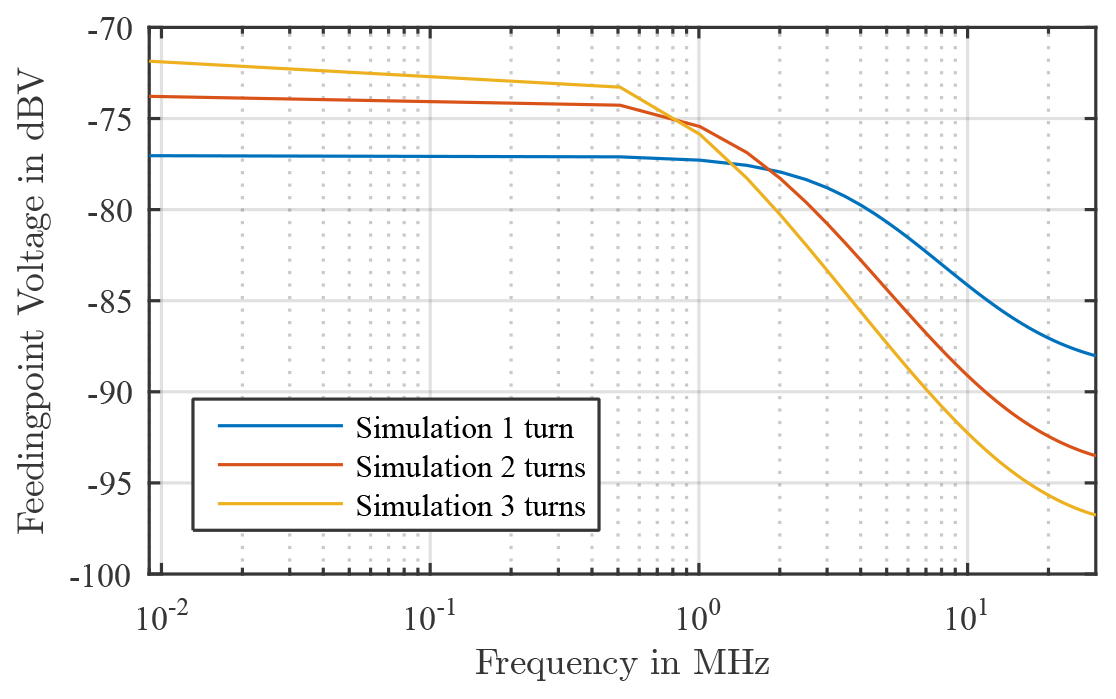
In Fig. 2 the result of the simulation is shown. The curve remains constant in the lower frequency range and decreases from a certain frequency with 20 dBV/dec​​​​​​​ and approaches a vertex in the high frequency range. Furthermore, it can be seen that with an increasing number of windings of the loop antenna, the higher the coupled field in the low frequency range. On the other hand, the course of the curve already decreases at a lower frequency and the vertexes is also lower in value with an increasing the number of winding.

Figure 2 Feedingpoint voltage of the Antennas with different numbers of windings.

3 Approaches to the realization of electrical equivalent circuit diagrams to validate the simulation results

In order to validate the results from the simulations, an equivalent circuit diagram (ECD) is modeled by numerical circuit calculation program. Two approaches are examined. One approach is to model a circuit from the ECD of a real coil and the second approach is to implement a circuit using the first resonance of the input impedance of the modeled antennas.

3.1 Approach of Equivalent circuit diagram from a Coil

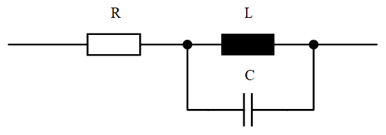
In order to validate the results from the simulations, an equivalent circuit diagram (ECD) is modeled in a numerical circuit calculation program. The basis for the ECD is a coil consisting of an ohmic resistor, which describes the wire losses and an inductance, which describes the self-inductance of the loop antenna. In addition, a capacitance is connected in parallel to the inductance, which describes the parasitic capacitances that arise between the individual windings and the wire sections of the loop antenna lying in parallel. Figure 3 shows the ECD of a real coil.

Figure 3 Electric equivalent circuit diagram from a Coil.

Following the modeling of the ECD, the individual components are calculated. The feedingpoint resistance of the receiving antenna is constant with 50 Ω for all simulations. The wire resistance can be determined as follows:

$$\begin{array}{}\text{(1)}& R={\displaystyle \frac{\mathit{\rho }l}{A}},\end{array}$$

where ρ is the specific resistance of the wire. In this case the value for copper is used. Furthermore, l stands for the length of the wire and from the number of windings. This results in the following calculation for the wire resistance:

$$\begin{array}{}\text{(2)}& R={\displaystyle \frac{\mathit{\rho }\cdot N\cdot \mathrm{2}\mathit{\pi }r}{A}}.\end{array}$$

Here represents N the number of windings and A is the cross-sectional area of the conductor. To calculate the parasitic capacitance, the simplified formula for calculating the capacitance of two parallel wires is assumed. According to Meinke and Gundlach (1992), the formula for the capacity is as follows:

$$\begin{array}{}\text{(3)}& C={\displaystyle \frac{\mathrm{2}\mathit{\pi }\mathit{\epsilon }l}{\ln \left(\frac{\mathrm{2}s}{D}+\sqrt{{\left(\frac{\mathrm{2}s}{D}\right)}^{\mathrm{2}}-\mathrm{1}}\right)}},\end{array}$$

Where l describes the length of the wire, s describes the distance between windings and D describes the wire diameter. For the different numbers of windings and the conductor loop used, the calculation of the parasitic winding capacitance results in:

$$\begin{array}{}\text{(4)}& C={\displaystyle \frac{\mathrm{2}\mathit{\pi }\mathit{\epsilon }\cdot \mathrm{2}\mathit{\pi }r}{(N-\mathrm{1})\cdot \ln \left(\frac{\mathrm{2}s}{D}+\sqrt{{\left(\frac{\mathrm{2}s}{D}\right)}^{\mathrm{2}}-\mathrm{1}}\right)}}.\end{array}$$

The inductance of the ECD is determined by the induction of a round wire loop, which Dengler (2016) described:

$$\begin{array}{}\text{(5)}& L=N^{\mathrm{2}}\mathit{\mu }\cdot r\cdot \left(\ln \left({\displaystyle \frac{\mathrm{8}r}{D}}\right)-\mathrm{2}+{\displaystyle \frac{Y}{\mathrm{2}}}+O\left({\displaystyle \frac{D^{\mathrm{2}}}{r^{\mathrm{2}}}}\right)\right),\end{array}$$

where Y is a constant that distinguishes whether the wire loop is a high or low frequency inductance. In this work a low-frequency inductance is assumed, where the current is evenly distributed over the wire cross-section. Hence $Y=\frac{\mathrm{1}}{\mathrm{2}}$, O can be neglected due to the relationship r≫D.

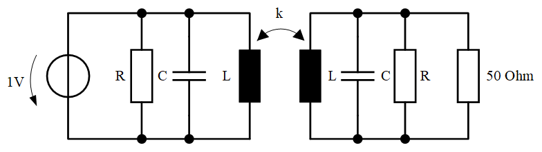
Both antennas from the simulation have been modeled exactly the same, which is why the two antennas also consist of the same components. The model of a transformer is used to take into account the coupling of the field into the receiving antenna. Here the coils are linked with a coupling factor. This is determined from the inductance of the two ECDs and the mutual inductance. This is determined from the geometric properties of the antennas and the distance between them. According to Wolff (1997), the mathematical expression of mutal inductance between two loops is as follows:

$$\begin{array}{}\text{(6)}& M={\displaystyle \frac{\mathit{\mu }{N}_{\mathrm{1}}{N}_{\mathrm{2}}}{\mathrm{4}\mathit{\pi }}}\cdot \underset{L_{\mathrm{1}}}{\int }\underset{L_{\mathrm{2}}}{\int }{\displaystyle \frac{\mathrm{d}{\mathit{s}}_{\mathbf{1}}\cdot \mathrm{d}{\mathit{s}}_{\mathbf{2}}}{|r_{\mathrm{1}}-r_{\mathrm{2}}|}}.\end{array}$$

The index denotes loop 1 and loop 2. For circular conductor loops, the mutual inductance can be simplified as follows:

$$\begin{array}{}\text{(7)}& M=\mathit{\mu }\cdot {\displaystyle \frac{N_{\mathrm{1}}{r}_{\mathrm{1}}^{\mathrm{2}}{N}_{\mathrm{2}}{r}_{\mathrm{2}}^{\mathrm{2}}\mathit{\pi }}{\mathrm{2}\sqrt{{\left(r_{\mathrm{1}}^{\mathrm{2}}+d^{\mathrm{2}}\right)}^{\mathrm{3}}}}}.\end{array}$$

Since both antennas are exactly the same, the circuit is simplified to:

$$\begin{array}{}\text{(8)}& M=\mathit{\mu }\cdot {\displaystyle \frac{N^{\mathrm{2}}{r}^{\mathrm{4}}\mathit{\pi }}{\mathrm{2}\sqrt{{\left(r^{\mathrm{2}}+d^{\mathrm{2}}\right)}^{\mathrm{3}}}}},\end{array}$$

where d represents the distance between the loop antennas. The coupling factor can be calculated from the mutual inductance and the two inductances as follows:

$$\begin{array}{}\text{(9)}& k={\displaystyle \frac{M}{\sqrt{L_{\mathrm{1}}{L}_{\mathrm{2}}}}}={\displaystyle \frac{M}{L}}.\end{array}$$

In Table 1 all values for the components of the ECD for the different numbers of windings are entered.

Table 1 Values of the individual components of the ECD for the different windings and their coupling factors.

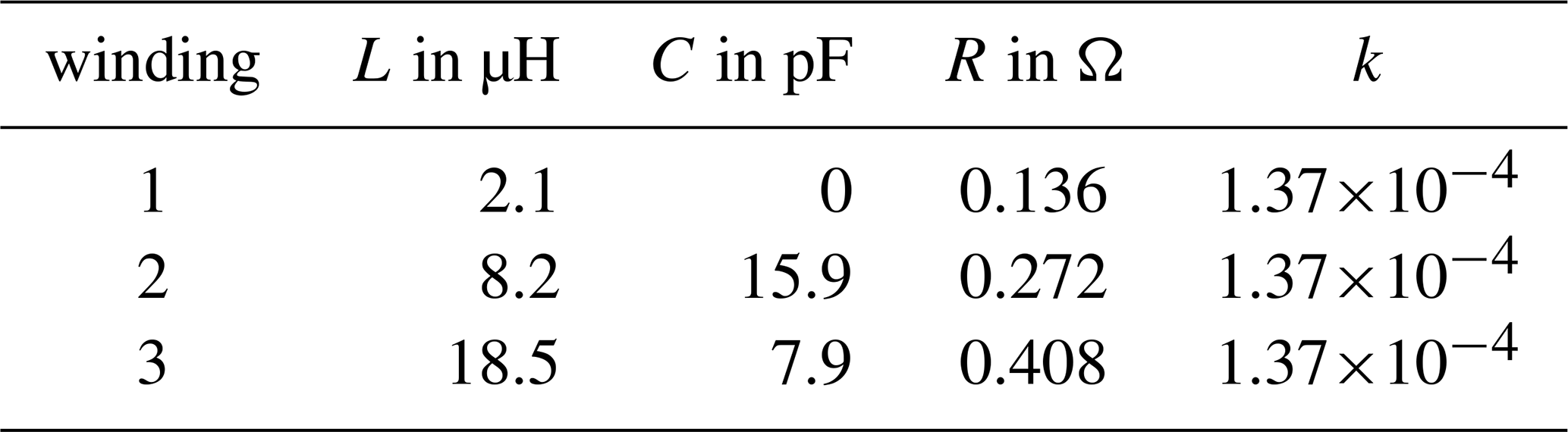
Figure 4 shows an example of the entired circuit for one winding, which was created in a numerical circuit calculation program. In this investigation, the feedingpoint voltage at an ohmic resistance of 50 Ω is determined. For this reason, the base resistance is connected in series with the ECD of the real coil in the second circuit. The source for the entire ECD is an ideal voltage source with 1 V in the first circuit.

Figure 4 Circuit created from the ECD of a real coil.

The results from the ECD, which can be seen in Fig. 5 in comparison with the results from the simulation, show a similarity in the courses to those from the field simulation. The course also remains mostly constant in the low frequency range and decreases from a certain frequency with 20 dBV/dec. Furthermore, it can also be seen that the higher the number of winding of the loop antenna, the higher the feedingpoint voltage is in the low frequency range. As well as the voltage drops even at a lower frequency. Furthermore, the voltage drops constantly up to the end of the frequency range, unlike the results from the simulation. This could be due to the ideal components and the calculation of the mutual inductance as well as the circuit simulation itself, since the spread of the magnetic field as a function of the frequency is not taken into account. Furthermore, it is noticeable that the amplitudes of the feedingpoint voltage are significantly lower and the frequency at which the voltage drops are lower than in the simulation.

Figure 5 Feedingpoint voltage determined from the ECD of a real Coil.

3.2 Approach of Equivalent circuit diagram from the first resonance of Input Impedance

The second approach for creating an ECD for the loop antennas is implemented from the input impedance of these antennas and based on the work of Kotzev et al. (2017). For this purpose, the input impedance was generated from the model in Concept II. Figure 6 shows the input impedance representative of antennas with one winding in the frequency range 1–1000 MHz.

Figure 6 Input impedance of the modeled antenna in Concept II.

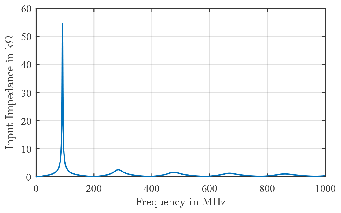
In the following, the determination of the individual components from the first resonance of the input impedance is presented, which can be described as a parallel resonant circuit. As can be seen in Fig. 6 the first resonance is approximately at a frequency of f₀= 91 MHz. Also it can determine the resistance, which is R=54 kΩ. The inductance can be determined in the low frequency part of the curve because of the following expression:

$$\begin{array}{}\text{(10)}& X(\mathit{\omega }\to \mathrm{0})\approx j\mathit{\omega }L.\end{array}$$

From this it follows to determine the inductance after changing the formula:

$$\begin{array}{}\text{(11)}& L=L(f\to \mathrm{0})\approx {\displaystyle \frac{X(f\to \mathrm{0})}{\mathrm{2}\mathit{\pi }f}}.\end{array}$$

To determine the capacitance, the formula for the resonance frequency depending on the inductance and capacitance is used. This is as follows:

$$\begin{array}{}\text{(12)}& f_{\mathrm{0}}={\displaystyle \frac{\mathrm{1}}{\mathrm{2}\mathit{\pi }\cdot \sqrt{LC}}}.\end{array}$$

This is adjusted according to the capacity C as follows:

$$\begin{array}{}\text{(13)}& C={\displaystyle \frac{\mathrm{1}}{\mathrm{4}{\mathit{\pi }}^{\mathrm{2}}{f}_{\mathrm{0}}^{\mathrm{2}}\cdot L}}.\end{array}$$

As in the first approach, the coupling of the magnetic field is also implemented using the model of a transformer. The coupling factor is calculated as follows:

$$\begin{array}{}\text{(14)}& k={\displaystyle \frac{M}{\sqrt{L_{\mathrm{1}}{L}_{\mathrm{2}}}}}={\displaystyle \frac{M}{L}}.\end{array}$$

The components for the circuits with two and three windings are determined analogously. In the Table 2 all values for the components of the circuit for the different numbers of windings are entered.

Table 2 Values of the individual components of the circuits for the different windings and their coupling factors.

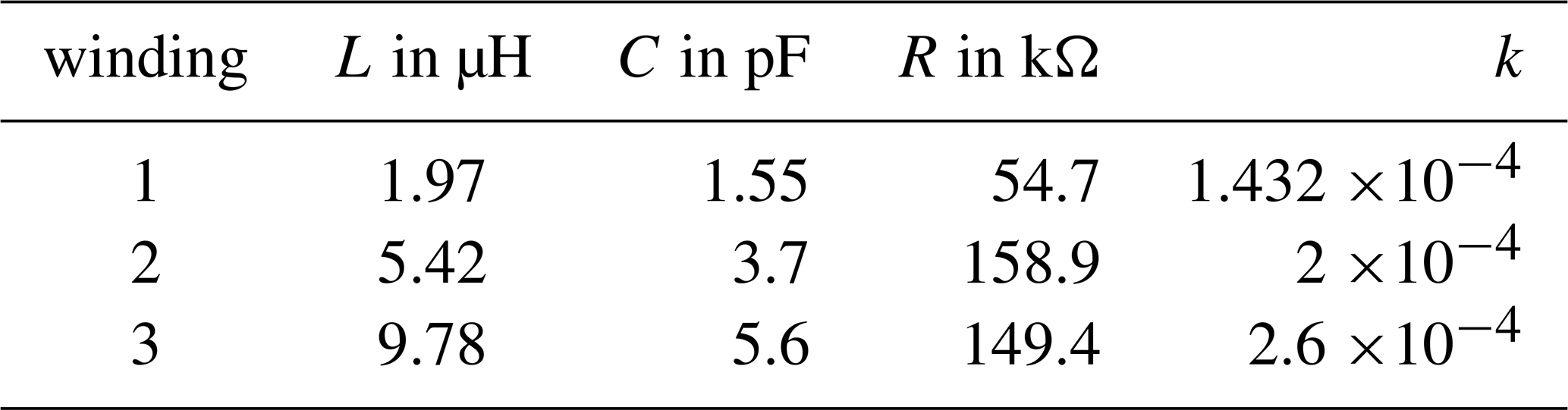
Figure 7 shows an example of the entire circuit for one winding, which was created in a numerical circuit calculation program.

Figure 7 Circuit created from the first resonance of the input impedance.

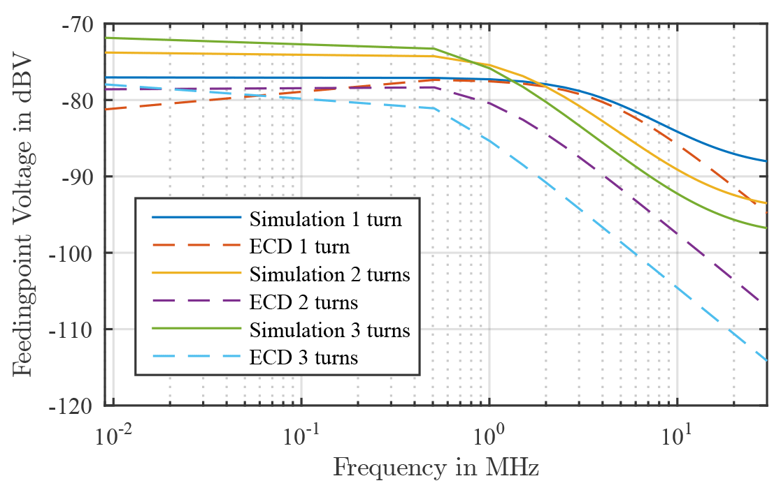
In Fig. 8 the results from the ECD of the input impedance can be seen in comparison with the results from the simulation and also show a clear similarity in the courses to those from the simulation and the previous approach. The same observations can be made here between the relationship between the height of the coupled-in field and the kink frequencies with the increasing number of windings. In this approach, however, the amplitudes and the kink frequencies match. The other one can also be seen here, then the voltage drops constantly in the higher frequency range. As already suspected in the previous approach, this could be due to the circuit simulation, since here the spread of the magnetic field as a function of the frequency is not taken into account. This will be examined further in the next chapter.

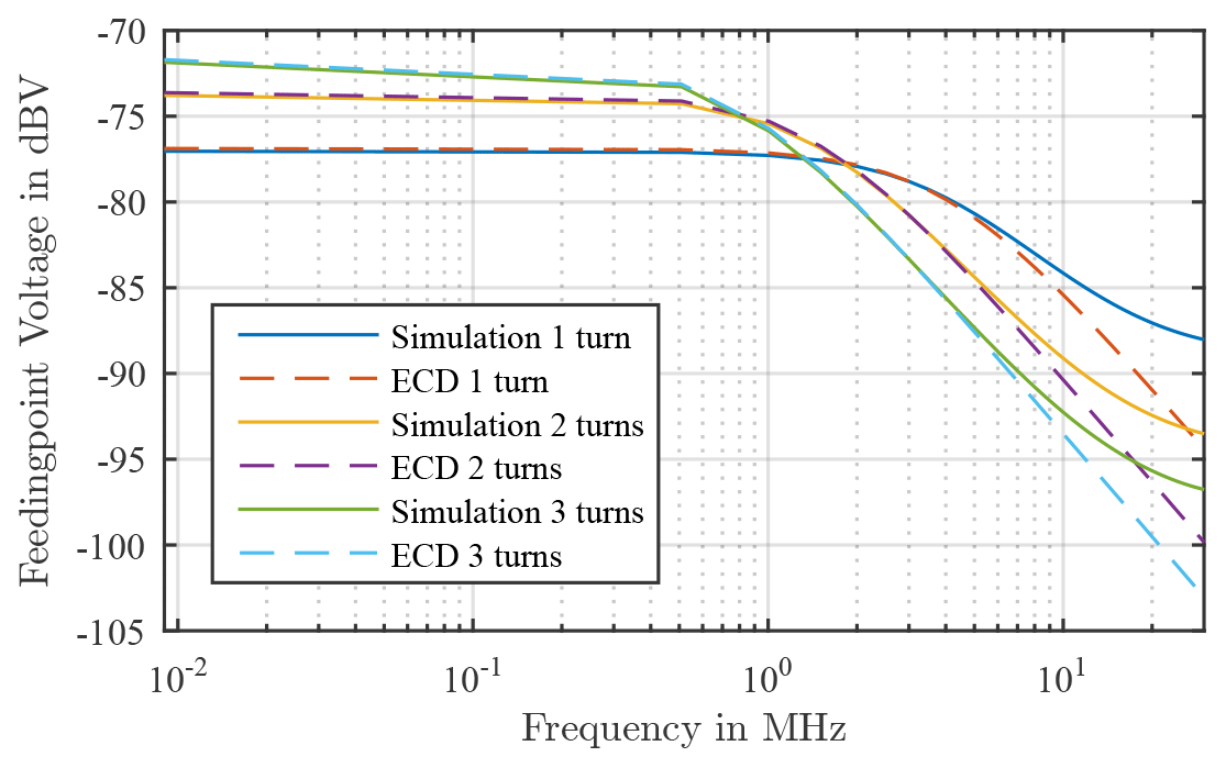
Figure 8 Feedingpoint voltage determined from the ECD of the first resonance of the input impedance.

4 Consideration of the Magnetic Field depending on Frequency

In the previous chapters, the mutual inductance was assumed to be a constant value from the geometry of the antennas and the distance. The mutual inductance is now examined as a function of the frequency.

Since the generator in the transmitting antenna supplies a constant voltage of 1 V and the input impedance and therefore the current flowing in the antenna depends on the frequency. The magnetic field resulting from the current as well as the magnetic flux density are therefore also dependent on the frequency. This is shown as follows:

$$\begin{array}{}\text{(15)}& \mathit{\Phi }=\underset{A}{\int }\mathit{\mu }\cdot H\mathrm{d}A.\end{array}$$

The mutual inductance depends on the magnetic flux density and the current and therefore also depends on the frequency:

$$\begin{array}{}\text{(16)}& M={\displaystyle \frac{\mathit{\Phi }}{I}}.\end{array}$$

Thus the relationship between magnetic field H, magnetic flux density Φ and mutual inductance M is proportional:

$$\begin{array}{}\text{(17)}& H\sim \mathit{\Phi }\sim M.\end{array}$$

The starting point is the magnetic field strength. This is determined with the help of the magnetic dipole method, since the simulation model describes a circular conductor loop. According to Henke (1992) the individual components of the magnetic field are determined as follows:

$$\begin{array}{}\text{(18)}& {\displaystyle }{H}_{\mathrm{r}}={\displaystyle \frac{\mathrm{2}\mathit{\pi }{r}^{\mathrm{2}}I{k}^{\mathrm{2}}}{\mathrm{4}\mathit{\pi }d}}\cdot \left({\displaystyle \frac{\mathrm{2}}{d^{\mathrm{2}}{k}^{\mathrm{2}}}}+j{\displaystyle \frac{\mathrm{2}}{dk}}\right)\cos \left(\mathrm{\Theta }\right)e^{j(\mathit{\omega }t-kd)}\text{(19)}& {\displaystyle }{H}_{\mathrm{\Theta }}={\displaystyle \frac{\mathrm{2}\mathit{\pi }{r}^{\mathrm{2}}I{k}^{\mathrm{2}}}{\mathrm{4}\mathit{\pi }d}}\cdot \left(-\mathrm{1}+{\displaystyle \frac{\mathrm{1}}{d^{\mathrm{2}}{k}^{\mathrm{2}}}}+j{\displaystyle \frac{\mathrm{1}}{dk}}\right)\sin \left(\mathrm{\Theta }\right)e^{j(\mathit{\omega }t-kd)}\text{(20)}& {\displaystyle }{H}_{\mathit{\Phi }}=\mathrm{0},\end{array}$$

where k describes the wavenumber. This can be determined by frequency and the speed of light as follows:

$$\begin{array}{}\text{(21)}& k={\displaystyle \frac{\mathrm{2}\mathit{\pi }f}{c}}.\end{array}$$

With a coaxial alignment the angle Θ to the surface normal z becomes 0. Thus the cosine of Θ is 1 and the sine of Θ is 0 and only the radial component of the magnetic field H_r has to be taken into account. Since only one point in space is considered over a frequency range, the time component can also be neglected. With these assumptions the magnetic field can be described as follows:

$$\begin{array}{}\text{(22)}& H_{\mathrm{r}}={\displaystyle \frac{\mathrm{4}\mathit{\pi }{r}^{\mathrm{2}}I{\left(\frac{\mathrm{2}\mathit{\pi }f}{c}\right)}^{\mathrm{2}}}{\mathrm{4}\mathit{\pi }d}}\cdot \left({\displaystyle \frac{\mathrm{1}}{d^{\mathrm{2}}{\left(\frac{\mathrm{2}\mathit{\pi }f}{c}\right)}^{\mathrm{2}}}}+j{\displaystyle \frac{\mathrm{1}}{d\left(\frac{\mathrm{2}\mathit{\pi }f}{c}\right)}}\right).\end{array}$$

The magnitude can be converted from the complex representation as follows:

$$\begin{array}{}\text{(23)}& \left|H_{\mathrm{r}}\right|={\displaystyle \frac{r^{\mathrm{2}}I{\left(\frac{\mathrm{2}\mathit{\pi }f}{c}\right)}^{\mathrm{2}}}{d}}\cdot \sqrt{{\left({\displaystyle \frac{\mathrm{1}}{d^{\mathrm{2}}{\left(\frac{\mathrm{2}\mathit{\pi }f}{c}\right)}^{\mathrm{2}}}}\right)}^{\mathrm{2}}+{\left({\displaystyle \frac{\mathrm{1}}{d\left(\frac{\mathrm{2}\mathit{\pi }f}{c}\right)}}\right)}^{\mathrm{2}}}.\end{array}$$

This magnitude of the magnetic field is determined in the considered frequency range of 9 kHz and 30 MHz. For this purpose, all variables are considered constant, so that r=0.5 m for the radius of the antenna, I=1 A for the current and d=3 m for the distance, since only the influence of the frequency is examined. Figure 9 shows the result of the frequency dependence of the magnetic field.

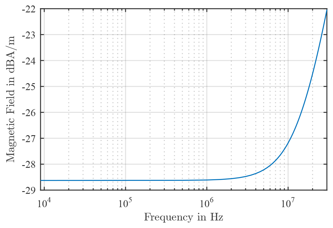
Figure 9 Magnetic field at a constant magnetic moment at a distance of 3 m depending on the frequency.

First, a constant curve can be seen in the lower frequency range. From a frequency around 10 MHz the magnetic field begins to rise by 20 dB/Dec. However, the focus here is not on the magnetic field, but the frequency dependency. As mentioned at the beginning, the magnetic field, the magnetic flux density and the mutual inductance are proportional to each another and also have the same frequency dependence. Therefore, the curve of the magnetic field is shifted to 0 dB in order to determine the influence of the frequency independently of all other variables. This acts like a kind of correction curve, while the frequency dependence of the magnetic field is not taken into account in the circuit simulation program with the ideal components. In Fig. 10 the frequency dependence shifted to 0 dB is shown.

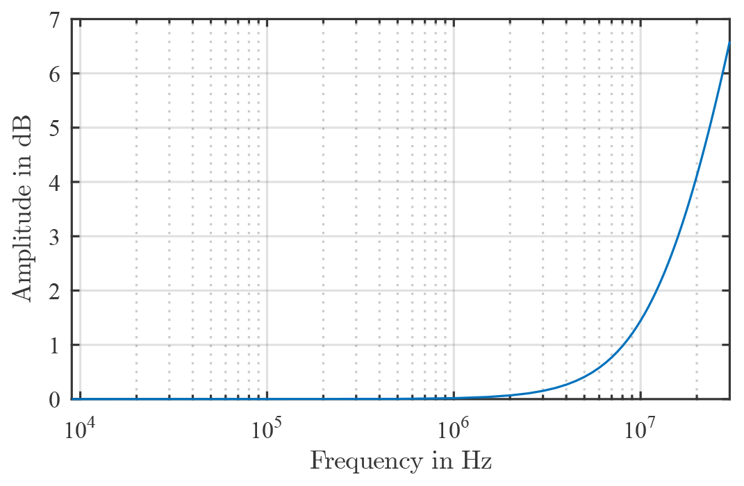
Figure 10 Correction curve to take into account the frequency dependence of the magnetic field.

This frequency dependency also applies to the mutual inductance M and must be added to this and thus the coupling capacitance also changes, since this is also proportional to the mutual inductance. Since no variable coupling factors can be set with the numerical circuit calculation program used, the frequency dependence was added to the already determined feedingpoint voltages. Since the voltages from the approach of the first resonance of the input impedance already showed better matches to the simulation, the frequency independence is added to these voltages. The results from this addition are shown in Fig. 11.

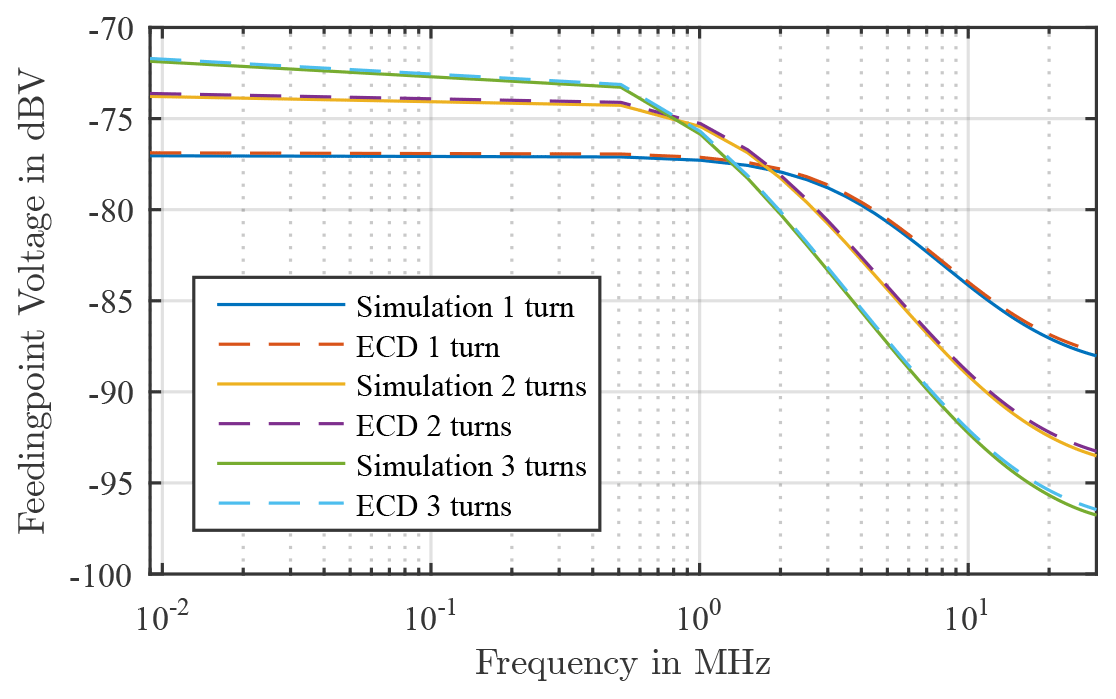
Figure 11 Comparison of the simulation results and the results also from the ECD, taking into account the frequency dependency.

These results show a very good agreement between the simulation and the results of the ECD. The results from the simulation can thus be validated analytically or with the help of an ECD with ideal components.

5 Conclusions

In this article, the results from the previous simulation should be validated. In the first step, a simulation of two loop antennas in the open space was modeled with a numerical field calculation program (Concept II) and the feedingpoint voltage was determined. To validate the simulation values, two approaches were then examined to confirm these results analytically and numerically with the aid of electrical equivalent circuit diagrams (ECD). These were modeled with a circuit simulator (LT-Spice). The focus here is on the mutual inductance of the two coils, which represents the coupling between the two antennas. In a first approach, the antenna was modeled as an ECD of a real coil, i.e. lossy with parasitic winding capacitance, and the individual components and mutual inductance were calculated analytically. The results showed a similar course to the results of the simulation. However, there were big differences in terms of the amplitudes of the voltage and in the higher frequency range the voltages continued to decrease, while those from the simulations approach a vertex. In a second approach, an ECD was modeled, which consists of the parallel resonance circuit of the first resonance of the antennas input impedance. The results from this approach agreed very well with the results from the simulation. However, the tensions continued to fall constantly. Therefore, in the next step, in addition to the constant mutual inductance, the influence of the frequency on the magnetic field and in winding on the coupling between the antennas was investigated. The analytic expression for the magnetic field was determined using the magnetic moment method and examined in the frequency range up to 30 MHz. A correction curve was then created from the results, which exclusively shows the frequency dependence of the magnetic field. Taking this correction curve into account, the feedingpoint voltage of the ECD was determined again from the second approach. This result corresponded very well with those from the simulation in the entire frequency range under consideration. Thus the results from the simulation could be validated analytically and numerically.