Pulse shaping of the electromagnetic radiation from a narrow slot antenna

A straightforward approach to achieve the prescribed shape of the far-field electromagnetic (EM) pulse radiated from a narrow slot antenna is introduced. It is demonstrated that the specified radiated pulse shape in a given direction can be approximately attained via a simple signal-processing technique that yields the pertaining excitation pulse. Illustrative numerical examples demonstrating good accuracy in the early-time part of the radiated pulsed fields are presented.

1 Introduction

Pulse shaping is in digital communication systems typically employed to reduce the bandwidth of a digital signal without jeopardizing its proper decoding at the receiver. Regarding an ultra-wide-band (UWB) radio link, an effort has been made to find the optimal excitation pulse shape to achieve the maximum amplitude, sharpness or energy of the received signal (Pozar, 2003; Liang and Xie, 2021). The overall performance of UWB systems is primarily limited by antennas that inevitably distort the pulse shape of the transmitted signal (Matila et al., 2004). Therefore, UWB antennas are designed with regard to the similarity between the shapes of radiated and excitation pulses, with the fidelity factor being one of the widely accepted quantitative performance indicators (Lamensdorf and Susman, 1994; Montoya and Smith, 1996; Quintero et al., 2011). Further optimization criteria may include maximization of the radiated amplitude at a given time and direction and maximization of the radiated energy density in a specified time interval (Pozar et al., 1984; Pozar, 2007).

In this article, a straightforward approach to control the pulse shape of the TD electric field radiated from a narrow slot antenna is presented. It is demonstrated that the specified radiated pulse shape in a given direction can be approximately achieved using a simple signal-processing technique that yields the pertaining excitation pulse. Although the presented analysis is limited to a narrow slot antenna, a similar line of reasoning is readily applicable to a relatively large class of antennas. The latter applies, in particular, to straight wire antennas for which the space-time electric-current distribution can be approximated by a series of causal, traveling (1+1)−D wave constituents (Tijhuis et al., 1992; Bogerd et al., 1998).

2 Problem definition

We shall analyze the transient EM radiation from a slot in a perfectly electrically conducting (PEC) plane (see Fig. 1). Position in the problem configuration is specified by the coordinates {x, y, z} with respect to a Cartesian reference frame with its origin, 𝒪, and the base vectors {i_x, i_y, i_z}. The position vector can be then expressed as $\mathit{r}=x{\mathit{i}}_x+y{\mathit{i}}_y+z{\mathit{i}}_z$. The time coordinate is t. Partial differentiation is denoted by ∂ that is supplemented with the pertaining subscript. The Heaviside unit-step function is denoted by H(t) and the Dirac-delta distribution is δ(t).

Figure 1 Narrow slot in a PEC screen excited by an impulsive electric-current source.

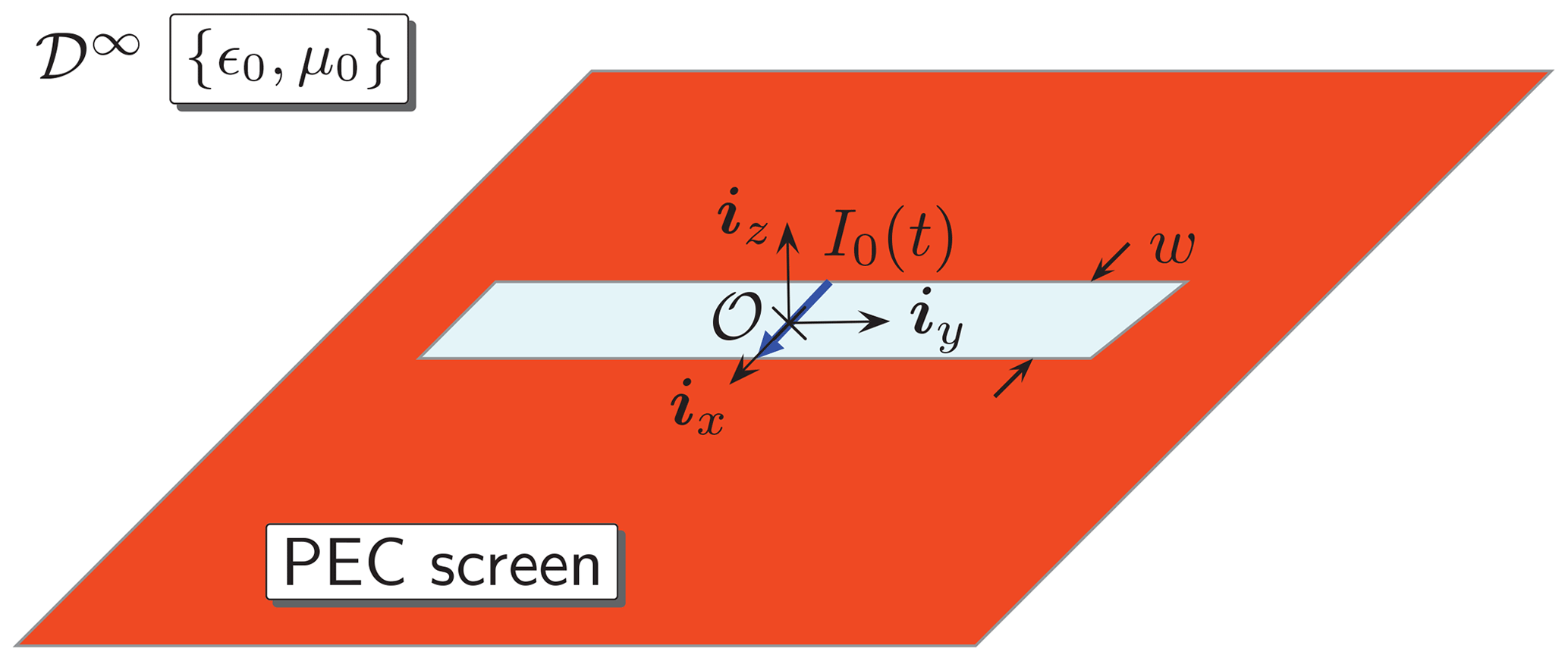
The slot occupies a bounded domain $\mathcal{S}=\mathit{\{}-w/\mathrm{2}<x<w/\mathrm{2}$, $-\mathrm{\ell }/\mathrm{2}<y<\mathrm{\ell }/\mathrm{2}$, z=0}, where w>0 and ℓ>0 denote its width and length, respectively. The slot's width is supposed to be relatively small. It is assumed that the slotted screen is located in free space, whose EM properties are described by electric permittivity ϵ₀ and magnetic permeability μ₀. The corresponding EM wave speed is $c_{\mathrm{0}}=({\mathit{ϵ}}_{\mathrm{0}}{\mathit{\mu }}_{\mathrm{0}}{)}^{-\mathrm{1}/\mathrm{2}}>\mathrm{0}$.

The slot is at its centre, y=0, and at t=0, activated by an x-oriented, localized electric-current source that is to be incorporated through a jump of the (y-component of the) magnetic-field strength, H_y, i.e.

$$\begin{array}{}\text{(1)}& \begin{array}{rl}{J}_{\mathrm{s}}(x,y,t)=& -H_y(x,y,z,t){|}_{z={\mathrm{0}}^{-}}^{{\mathrm{0}}^{+}}=I_{\mathrm{0}}\left(t\right)\mathit{\delta }\left(y\right)\\ & \mathrm{for}\mathit{\{}-w/\mathrm{2}<x<w/\mathrm{2}\mathit{\}}\mathrm{and}t>\mathrm{0},\end{array}\end{array}$$

where I₀(t) is the (causal) electric-current excitation pulse and J_s denotes (the x-component of) the equivalent electric-current surface density. It is assumed that prior to t=0 the EM fields in the configuration vanish identically. Accordingly, its one-sided Laplace transform is written as

$$\begin{array}{}\text{(2)}& {\widehat{I}}_{\mathrm{0}}\left(s\right)=\underset{t=\mathrm{0}}{\overset{\mathrm{\infty }}{\int }}\exp (-st)I_{\mathrm{0}}\left(t\right)\mathrm{d}t,\end{array}$$

where s is the Laplace-transform parameter (= complex frequency) with ℜ(s)>0.

Owing to the relatively small width, the equivalent magnetic-current surface density induced in the slot is essentially concentrated along the slot's axis. The induced voltage distribution, say V(y,t), induced across the slot can be then related to the corresponding electric-field strength, E_x, via $V(y,t)=-w{E}_x(\mathrm{0},y,\mathrm{0},t)$. The pulsed EM-field radiation from the slot can be attributed to the induced voltage, the space-time distribution of which is attainable via the Cagniard–deHoop method of moments (CdH-MoM) (Štumpf, 2022, Sect. 13.3), for example. It is noted that for a piecewise-linear space-time distribution of the electric-current-excited voltage response, the corresponding “aperture TD admittance matrix” has been derived analytically in the form of elementary functions only (Štumpf, 2022, Sect. 13.3.2).

3 Approximate radiation model

The TD EM field as radiated from the slot antenna can be in the far-field region expanded as (de Hoop, 1995, Sect. 26.12)

$$\begin{array}{}\text{(3)}& \begin{array}{rl}{\mathit{E}}^{\mathrm{T}}(\mathit{r},t)=& {\displaystyle \frac{{\mathit{E}}^{\mathrm{T};\mathrm{\infty }}\left(\mathit{\xi },t-\left|\mathit{r}\right|/c_{\mathrm{0}}\right)}{\mathrm{4}\mathit{\pi }\left|\mathit{r}\right|}}\left[\mathrm{1}+O\left(|\mathit{r}{|}^{-\mathrm{1}}\right)\right]\\ & \mathrm{as}\left|\mathit{r}\right|\to \mathrm{\infty },\end{array}\end{array}$$

where ${\mathit{E}}^{\mathrm{T};\mathrm{\infty }}(\mathit{\xi },t)$ is the electric-field amplitude radiation characteristic and $\mathit{\xi }=\mathit{r}/\left|\mathit{r}\right|$ denotes the unit vector in the direction of observation. In accordance with the TD source-type representations applying to a homogeneous, isotropic and lossless background medium (de Hoop, 1995, Sect. 26.4), the TD EM near- and intermediate-field radiated components that are proportional to $|\mathit{r}{|}^{-\mathrm{3}}$ and $|\mathit{r}{|}^{-\mathrm{2}}$, respectively, can be far away from the antenna neglected. Equation (3) further shows that the EM field radiated from the slot antenna has the form of a radially expanding spherical wave. The TD amplitude radiation characteristic is a function of ξ and t only, and can be, in fact, related to the Radon transform of the (time-differentiated) magnetic-current surface density induced in the slot (de Hoop et al., 2009, Appendix B). For the sake of simplicity, we shall further limit our analysis to the radiated electric field at ξ=i_z. Along the boresight axis, its z-component is zero, the y-component is relatively small, while the (dominant) x-component can be expressed using the induced voltage as

$$\begin{array}{}\text{(4)}& E_x^{\mathrm{T};\mathrm{\infty }}\left({\mathit{i}}_z,t\right)=-\mathrm{2}{c}_{\mathrm{0}}^{-\mathrm{1}}{\partial }_t\underset{y^{\prime }=-\mathrm{\ell }/\mathrm{2}}{\overset{\mathrm{\ell }/\mathrm{2}}{\int }}V(y^{\prime },t)\mathrm{d}{y}^{\prime }.\end{array}$$

For the piecewise-linear spatial distribution assumed in the CdH-MoM solution, the standard trapezoidal rule can be applied to evaluate the spatial integration in Eq. (4) exactly. Our (inverse) objective, however, is to find the excitation current I₀(t) that leads to the prescribed radiated field. Under the assumption that the far-field radiation is not sensitive to a first-order error in the source voltage distribution, we shall suppose that the latter can be approximately determined through a simple transmission-line (TL) model that is specified by a system of coupled equations

$$\begin{array}{}\text{(5)}& {\displaystyle }& {\displaystyle }{\partial }_{y}V(y,t)+L{\partial }_{t}I(y,t)=\mathrm{0},\text{(6)}& {\displaystyle }& {\displaystyle }{\partial }_{y}I(y,t)+C{\partial }_{t}V(y,t)=\mathrm{0},\end{array}$$

and supplemented with the excitation and end conditions

$$\begin{array}{}\text{(7)}& {\displaystyle }& \begin{array}{c}\lim \\ y\downarrow \mathrm{0}\end{array}I(y,t)-\begin{array}{c}\lim \\ y\uparrow \mathrm{0}\end{array}I(y,t)=I_{\mathrm{0}}\left(t\right),\text{(8)}& {\displaystyle }& {\displaystyle }V(\pm \mathrm{\ell }/\mathrm{2},t)=\mathrm{0},\end{array}$$

respectively, for all t>0. At the expense of additional complexities, more sophisticated traveling-wave models would incorporate (s-dependent) reflections at the ends of the slot, as well as (s-dependent) loss mechanisms. Upon solving Eqs. (5)–(8) (see Appendix A), the resulting voltage distribution can be substituted in Eq. (4), which leads to

$$\begin{array}{}\text{(9)}& \begin{array}{rl}{E}_x^{\mathrm{T};\mathrm{\infty }}& \left({\mathit{i}}_z,t\right)\simeq -\mathrm{2}\mathit{\zeta }\sum _{n=\mathrm{0}}^{\mathrm{\infty }}\left\{I_{\mathrm{0}}(t-\mathrm{2}nT)\right.\\ & -I_{\mathrm{0}}[t-\mathrm{2}(n+\mathrm{1}\left)T\right]+\mathrm{2}{I}_{\mathrm{0}}[t-(\mathrm{3}T/\mathrm{2}+\mathrm{2}nT\left)\right]\\ & \left.-\mathrm{2}{I}_{\mathrm{0}}[t-(T/\mathrm{2}+\mathrm{2}nT\left)\right]\right\}\exp (-\mathit{\alpha }t),\end{array}\end{array}$$

where $T=\mathrm{\ell }/c_{\mathrm{0}}$ is the travel time, $\mathit{\zeta }=(L/C{)}^{\mathrm{1}/\mathrm{2}}$ denotes the impedance parameter, and we incorporated, in addition, the exponential decay with constant α>0. Using Eq. (9) we interrelated the radiated TD field with the excitation current in a simple manner. It should be noted that the methodology that led to Eq. (9) does not have to be limited to the boresight radiation. In fact, the TD radiation characteristics at a slanting direction can be represented via the Radon transformation (Fokkema and van den Berg, 1993, Sect. 1.2.2) that can still be handled for the TL approximation analytically. Thanks to the property of causality, I₀(t)=0 for t<0, the number of terms in the sum is always finite. Moreover, this property makes it possible to apply the time translation rule of the Laplace transformation (Abramowitz and Stegun, 1972, Eq. (29.2.15)) and cast the s-domain image of the excitation current into the following form (see Appendix B, for more details)

$$\begin{array}{}\text{(10)}& {\widehat{I}}_{\mathrm{0}}\left(s\right)=\widehat{\mathrm{\Psi }}\left(s\right)/\widehat{\mathrm{\Delta }}\left(s\right),\end{array}$$

where $\widehat{\mathrm{\Psi }}\left(s\right)$ denotes the s-domain image of Ψ(t) that is closely related to the (prescribed) radiated electric-field signal via

$$\begin{array}{}\text{(11)}& {\displaystyle }& {\displaystyle }\mathrm{\Psi }\left(t\right)=\mathrm{\Phi }\left(t\right)-\mathrm{\Phi }(t-\mathrm{2}T),\text{(12)}& {\displaystyle }& {\displaystyle }\mathrm{\Phi }\left(t\right)=-E_x^{\mathrm{T};\mathrm{\infty }}\left({\mathit{i}}_z,t\right)\exp \left(\mathit{\alpha }t\right)/\mathrm{2}\mathit{\zeta },\end{array}$$

and, the denominator reads

$$\begin{array}{}\text{(13)}& \begin{array}{rl}\widehat{\mathrm{\Delta }}\left(s\right)& =\mathrm{1}-\exp (-\mathrm{2}sT)\\ & -\mathrm{2}\exp (-sT/\mathrm{2})+\mathrm{2}\exp (-\mathrm{3}sT/\mathrm{2}).\end{array}\end{array}$$

The inverse transform of Eq. (10) can be carried out analytically using the (convergent) Taylor series about $\left|s\right|\to \mathrm{\infty }$, i.e.

$$\begin{array}{}\text{(14)}& {\displaystyle \frac{\mathrm{1}}{\widehat{\mathrm{\Delta }}\left(s\right)}}=\sum _{n=\mathrm{0}}^{\mathrm{\infty }}{w}_n\exp (-snT/\mathrm{2}),\end{array}$$

with $w_n=\left[\mathrm{2}\right(n+\mathrm{2}{)}^{\mathrm{2}}-\mathrm{1}+(-\mathrm{1}{)}^{n+\mathrm{2}}]/\mathrm{8}$. Substituting then Eq. (14) in Eq. (10) and transforming the resulting terms via the time translation rule (Abramowitz and Stegun, 1972, Eq. (29.2.15)) to the TD, we finally end up with (cf. Eq. 9)

$$\begin{array}{}\text{(15)}& I_{\mathrm{0}}\left(t\right)=\sum _{n=\mathrm{0}}^{\mathrm{\infty }}{w}_n\mathrm{\Psi }(t-nT/\mathrm{2}).\end{array}$$

Equation (15) with Eqs. (11) and (12) gives the excitation electric-current pulse in terms of (scaled and shifted) copies of the desired radiated field. The TL model parameters ζ and α are as yet unknown and can be, for a particular slot antenna, readily determined through a numerical experiment. The entire solution procedure is demonstrated and validated in the following section.

4 Numerical example

Throughout this section, we shall analyze the pulsed EM radiation from a slot of dimensions w=1.0 mm and ℓ=100 mm. The solution methodology consists of three steps:

• determination of α and ζ parameters of the simplified radiation model (via Eq. 9);

• calculation of I₀(t) using Eq. (15) for a desired $E_x^{\mathrm{T};\mathrm{\infty }}({\mathit{i}}_z,t)$;

• calculation of the actual $E_x^{\mathrm{T};\mathrm{\infty }}({\mathit{i}}_z,t)$ using the excitation pulse from the previous step.

First, we shall determine the parameters α and ζ of the simplified TL radiation model. To that end, the antenna is excited by a chosen electric-current pulse and the pertaining radiated electric field is calculated using both an available EM-field solver and Eq. (9). For this purpose, we used our CdH-MoM MATLAB^® code and found that Eq. (9) with ζ=120 Ω and $\mathit{\alpha }=\mathrm{0.20}/T$ yields satisfactory estimates of the radiated field. The accuracy of the TL model can be illustrated for an excitation pulse of the bipolar-triangle shape, for example. Accordingly, we take

$$\begin{array}{}\text{(16)}& I_{\mathrm{0}}\left(t\right)=I_{\mathrm{m}}f\left(t\right),\end{array}$$

with

$$\begin{array}{}\text{(17)}& \begin{array}{rl}f\left(t\right)& ={\displaystyle \frac{\mathrm{2}}{t_{\mathrm{w}}}}\left[tH\left(t\right)-\mathrm{2}\left(t-{\displaystyle \frac{t_{\mathrm{w}}}{\mathrm{2}}}\right)H\left(t-{\displaystyle \frac{t_{\mathrm{w}}}{\mathrm{2}}}\right)\right.\\ & \left.+\mathrm{2}\left(t-{\displaystyle \frac{\mathrm{3}{t}_{\mathrm{w}}}{\mathrm{2}}}\right)H\left(t-{\displaystyle \frac{\mathrm{3}{t}_{\mathrm{w}}}{\mathrm{2}}}\right)-\left(t-\mathrm{2}{t}_{\mathrm{w}}\right)H\left(t-\mathrm{2}{t}_{\mathrm{w}}\right)\right],\end{array}\end{array}$$

where I_m=1.0 A and c₀t_w=ℓ. Figure 2 shows the resulting pulse shapes in the bounded time window $\mathit{\{}\mathrm{0}\le c_{\mathrm{0}}t/\mathrm{\ell }\le \mathrm{6}\mathit{\}}$. For validation purposes, the TD radiated field has also been evaluated using the finite-integration technique (FIT) as implemented in CST Studio Suite^®. As can be observed, the calculated signals correlate well.

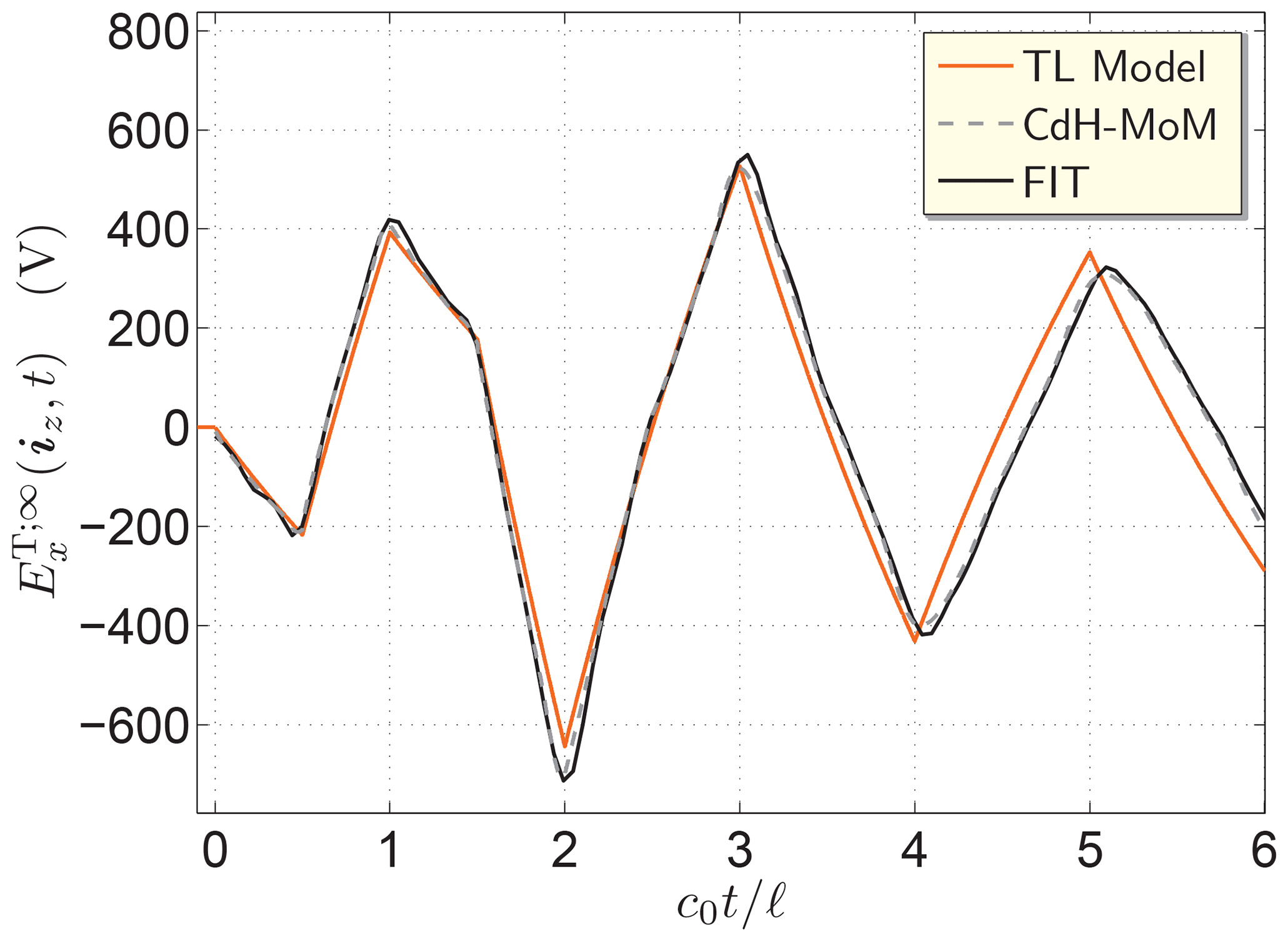
Figure 2 The TD electric-field amplitude radiated from the analyzed slot of dimensions w=1.0 mm and ℓ=100 mm. The pulses were calculated via the simplified TL model (Eq. 9) with ζ=20 Ω and $\mathit{\alpha }=\mathrm{0.20}/T$, and numerically using CdH-MoM and FIT.

Second, with the parameters of the TL radiation model at our disposal, we may apply Eq. (15) to calculate the excitation pulse shape, I₀(t), for a specified TD radiated field. As an example, we may wish to radiate the bipolar triangle pulse that proved to be capable of probing the shape of a 3-D scatterer (Štumpf, 2014). Accordingly, the desired pulse shape of the radiated electric field is described by

$$\begin{array}{}\text{(18)}& E_x^{\mathrm{T};\mathrm{\infty }}\left({\mathit{i}}_z,t\right)=V_{\mathrm{m}}f\left(t\right),\end{array}$$

where we take V_m=100 V and c₀t_w=ℓ, for example. The corresponding electric-current excitation pulse as found via Eq. (15) is shown in Fig. 3a.

Third, using the thus calculated excitation pulse, the CdH-MoM (or/and FIT) can be applied to calculate the corresponding TD radiated electric field. The pertaining TD response is shown in Fig. 3b. As a reference, we also plot the “ideal” pulse calculated via Eq. (9) that agrees with the desired one (see Eq. 18), as expected.

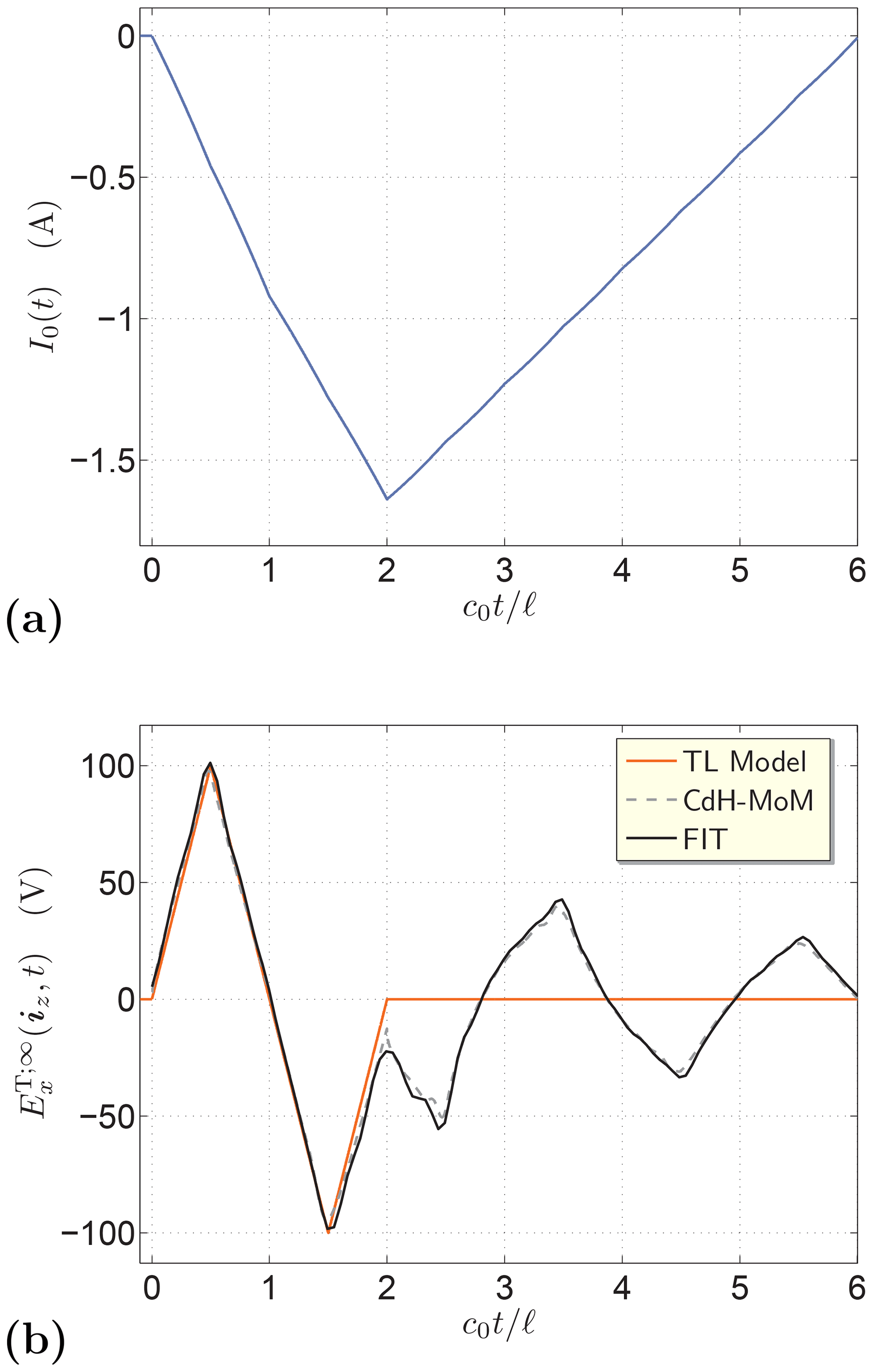
Figure 3 (a) Excitation electric-current pulse and (b) the corresponding TD radiated fields at ξ=i_z. The “ideal” signal was calculated via Eq. (9) and the “actual” one with the aid of CdH-MoM and FIT.

While its early-time part is reproduced very well, the actual TD radiated field exhibits typical “ringing” that spreads the TD response. This dominantly unwanted effect could be in part compensated, at the expense of deteriorating the radiation efficiency, by a resistive loading (Matila et al., 2004). Such an additional attenuation can be then approximately incorporated in the TL radiation model through an increase of the exponential decay constant α (see Eq. 9). The observation that the inverse methodology is less accurate in the late-time part of the TD response could be deduced already from Fig. 2 where it is seen that the TL approximation gets worse as time passes. This effect can largely be attributed to the relatively crude approximation of reflections at the ends of the slot (see Eq. 8). Consequently, in a fixed time window of observation, the accumulated error due to multiple reflections can also be reduced by extending the (relative) length of the slot.

The presented methodology can be readily generalized. Indeed, we may then prescribe, for example, a relatively short triangular pulse with V_m=100 V and $c_{\mathrm{0}}{t}_{\mathrm{w}}=\mathrm{\ell }/\mathrm{2}$ (see Eq. 18 with Eq. 17) to be radiated at a slanting direction, say $\mathit{\xi }={\mathit{\xi }}_{\mathrm{0}}=\sin (\mathit{\pi }/\mathrm{6}){\mathit{i}}_y+\cos (\mathit{\pi }/\mathrm{6}){\mathit{i}}_z$. The pertaining excitation signal along with the ideal and actual radiated pulse shapes are shown in Fig. 4. It is seen that the initial part of the TD response is again reproduced well.

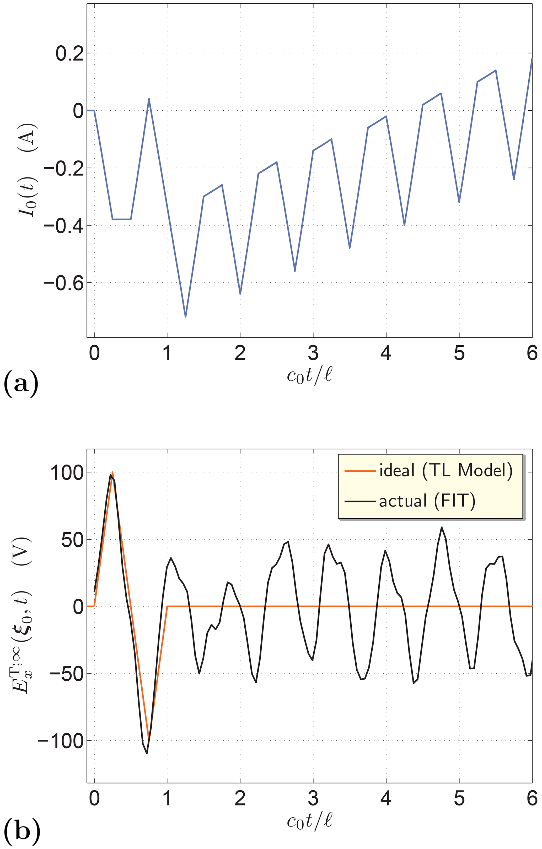
Figure 4 (a) Excitation electric-current pulse and (b) the corresponding TD radiated fields at $\mathit{\xi }={\mathit{\xi }}_{\mathrm{0}}=\sin (\mathit{\pi }/\mathrm{6}){\mathit{i}}_y+\cos (\mathit{\pi }/\mathrm{6}){\mathit{i}}_z$.

It is finally noted that the introduced expression for the excitation pulse (Eq. 15) can also serve as the initial estimate for iterative optimization algorithms (Kelley, 1999) that may further improve the results. Their use, however, requires multiple solutions of the (direct) antenna radiation problem, which can be computationally expensive. On the other hand, the evaluation of our closed-form result (Eq. 15) is virtually effortless.

5 Conclusions

We have introduced a straightforward methodology that enables to control the pulsed EM-field radiation from a narrow slot antenna. The solution approach relies on the approximation of the TD radiated field in the form of a sum of time-delayed and scaled copies of the excitation pulse, a form that can be solved for the excitation pulse analytically. Illustrative examples demonstrate that the solution approach is capable of achieving the desired radiated pulse with a good accuracy, in particular, at its early-time part. The presented methodology is easy-to-implement, which makes it suitable for providing initial estimates in more advanced inverse procedures.

Appendix A: Transmission-line model

The solution of the TL problem specified via Eqs. (5)–(8) can be written in terms of traveling-wave constituents according to

$$\begin{array}{}\text{(A1)}& V(y,t)=\sum _{n=\mathrm{0}}^{\mathrm{\infty }}{V}^{\left[n\right]}(y,t),\end{array}$$

where

$$\begin{array}{}\text{(A2)}& \begin{array}{rl}{V}^{\left[n\right]}(y,t)& ={\displaystyle \frac{\mathrm{1}}{\mathrm{2}}}\mathit{\zeta }\mathit{\{}{I}_{\mathrm{0}}\left(t-y/c_{\mathrm{0}}-\mathrm{2}nT\right)\\ & -I_{\mathrm{0}}\left[t+y/c_{\mathrm{0}}-(\mathrm{2}n+\mathrm{1})T\right]\\ & +I_{\mathrm{0}}\left[t+y/c_{\mathrm{0}}-\mathrm{2}(n+\mathrm{1})T\right]\\ & -I_{\mathrm{0}}\left[t-y/c_{\mathrm{0}}-(\mathrm{2}n+\mathrm{1})T\right]\mathit{\}}\end{array}\end{array}$$

for all $\mathit{\{}\mathrm{0}\le y\le \mathrm{\ell }/\mathrm{2}\mathit{\}}$ and t>0, with $T=\mathrm{\ell }/c_{\mathrm{0}}$ and $\mathit{\zeta }=(L/C{)}^{\mathrm{1}/\mathrm{2}}$, and, similarly,

$$\begin{array}{}\text{(A3)}& \begin{array}{rl}{V}^{\left[n\right]}(y,t)& ={\displaystyle \frac{\mathrm{1}}{\mathrm{2}}}\mathit{\zeta }\mathit{\{}{I}_{\mathrm{0}}\left(t+y/c_{\mathrm{0}}-\mathrm{2}nT\right)\\ & -I_{\mathrm{0}}\left[t-y/c_{\mathrm{0}}-(\mathrm{2}n+\mathrm{1})T\right]\\ & +I_{\mathrm{0}}\left[t-y/c_{\mathrm{0}}-\mathrm{2}(n+\mathrm{1})T\right]\\ & -I_{\mathrm{0}}\left[t+y/c_{\mathrm{0}}-(\mathrm{2}n+\mathrm{1})T\right]\mathit{\}}\end{array}\end{array}$$

for all $\mathit{\{}-\mathrm{\ell }/\mathrm{2}\le y\le \mathrm{0}\mathit{\}}$ and t>0. These expressions have been substituted in Eq. (4) to get the approximate expression (Eq. 9) for the radiated, TD electric-field amplitude. To keep the approximate radiation model simple, its losses were incorporated via the exponential decay factor exp (−αt), where α is an s-independent positive constant (see Eq. 9). As a matter of fact, this corresponds to replacing s with s+α in (the s-domain counterparts of) the right-hand sides of Eqs. (A2) and (A3) (see Abramowitz and Stegun, 1972, Eq. (29.2.12)). This sort of approximation is commonly used in the literature on the subject (e.g., Šesnić et al., 2011).

Appendix B: Inversion procedure

The approximate expression for the TD radiated amplitude based on the TL model (see Appendix A) can readily be transformed to the s-domain using the time translation rule of the Laplace transform (Abramowitz and Stegun, 1972, Eq. (29.2.15)). Following this way, we obtain

$$\begin{array}{}\text{(B1)}& {\widehat{E}}_x^{\mathrm{T};\mathrm{\infty }}\left({\mathit{i}}_z,s\right)\simeq -\mathrm{2}\mathit{\zeta }{\widehat{I}}_{\mathrm{0}}\left(s\right)\widehat{\mathrm{\Delta }}\left(s\right)\sum _{n=\mathrm{0}}^{\mathrm{\infty }}\exp (-\mathrm{2}snT),\end{array}$$

and recall that $\widehat{\mathrm{\Delta }}\left(s\right)$ is defined by Eq. (13). As for practical applications we may restrict ourselves to causal and bounded signals, Eq. (B1) makes sense for all ℜ(s)>0. With such transform parameters, the geometric-series expansion,

$$\begin{array}{}\text{(B2)}& \sum _{n=\mathrm{0}}^{\mathrm{\infty }}\exp (-\mathrm{2}snT)={\displaystyle \frac{\mathrm{1}}{\mathrm{1}-\exp (-\mathrm{2}sT)}},\end{array}$$

is convergent, and can be hence used in Eq. (B1) to get a straightforward s-domain expression from which ${\widehat{I}}_{\mathrm{0}}\left(s\right)$ immediately follows as

$$\begin{array}{}\text{(B3)}& {\widehat{I}}_{\mathrm{0}}\left(s\right)=-{\displaystyle \frac{{\widehat{E}}_x^{\mathrm{T};\mathrm{\infty }}\left({\mathit{i}}_z,s\right)}{\mathrm{2}\mathit{\zeta }}}{\displaystyle \frac{\mathrm{1}-\exp (-\mathrm{2}sT)}{\widehat{\mathrm{\Delta }}\left(s\right)}}.\end{array}$$

Finally, using of the (convergent) series expansion (Eq. 14) in Eq. (B3), we get

$$\begin{array}{}\text{(B4)}& \begin{array}{rl}{\widehat{I}}_{\mathrm{0}}\left(s\right)& =-{\displaystyle \frac{{\widehat{E}}_x^{\mathrm{T};\mathrm{\infty }}\left({\mathit{i}}_z,s\right)}{\mathrm{2}\mathit{\zeta }}}[\mathrm{1}-\exp (-\mathrm{2}sT\left)\right]\\ & \times \sum _{n=\mathrm{0}}^{\mathrm{\infty }}{w}_n\exp (-snT/\mathrm{2}),\end{array}\end{array}$$

which has the form that is amenable to the analytical Laplace inversion via (Abramowitz and Stegun, 1972, Eq. (29.2.15)).