 | 21 Mar 2023
Measurement and transformation of continuously modulated fields using a short-time measurement approach
Jana Daubmeier
Thomas F. Eibert
Near-field measurements, which are performed in-situ, may suffer from the fact that the antenna under test (AUT) cannot be accessed to transmit or receive a specifically tailored test signal. In some scenarios, it might also be desired to test the AUT during its real operation state, especially when it comes to the verification of antenna systems. Therefore, the need to handle time- and space-modulated fields in combination with a time-harmonic near-field to far-field transformation (NFFFT) arises. For the case where unmanned aerial vehicles (UAVs) carry the field probe in in-situ measurement scenarios, long observation times, required for the resolution of the frequency spectra of modulated fields, are detrimental due to the UAV movement resulting in blurred measurement positions. The short-time measurement (STM) approach, presented in this article, offers a way to transform the measured field data using a time-harmonic NFFFT with short observation times for the collection of the individual field samples. Measurements are shown which demonstrate the applicability of the STM approach for the measurement and transformation of continuously time-modulated fields in different measurement scenarios.
- Article
(2159 KB) - Full-text XML
- BibTeX
- EndNote


In recent years, the field of in-situ antenna measurements has gained considerable interest towards the determination of far-field (FF) radiation patterns as one of the most important characteristics of any antenna. Beside measuring the FF directly, near-field (NF) measurements in combination with a subsequent near-field to far-field transformation (NFFFT) are an established technique for the characterization of antennas (Paris et al., 1978; Yaghjian, 1986). Commonly, NF measurements are performed in anechoic chambers as they provide a controlled environment, which is a good approximation of free space. In-situ measurements, in contrast, open up new opportunities since the characterization of large or mounted antennas becomes realistic, even with the consideration of their real operating environment. There have been many approaches for the realization of in-situ antenna measurements, e.g., where an operator person moves the field probe (He et al., 2016; Faul et al., 2020) or, more sophisticated, by the use of an overhead crane (Geise et al., 2019). The most promising realization, however, is to carry the field probe by an unmanned aerial vehicle (UAV). Moreover, the development in the field of in-situ antenna measurements was elevated by the availability of advanced NFFFT algorithms, which offer advanced features such as the suppression of scatterers (Yinusa and Eibert, 2013; Eibert et al., 2015) or the consideration of dielectric and lossy ground (Mauermayer and Eibert, 2018). Antenna measurements with UAVs have been demonstrated for various frequency ranges (Paonessa et al., 2016; García-Fernández et al., 2017; Faul and Eibert, 2021a) and for applications such as the measurement of mobile radio base stations (Fernandez et al., 2018) or radio navigation signals (Schrader et al., 2019; Sommer et al., 2020). Specifically in the field of radio navigation, UAV-based antenna measurements can have a significant impact, when it comes to the verification of navigational aids (NAVAIDs) for aviation. Due to the high safety standards in aviation, NAVAIDs such as the instrument landing system (ILS) or the VHF omnidirectional radio range (VOR) have to be checked on a regular basis according to the requirements of the International Civil Aviation Organization (ICAO). Up to now, the validation of the correct operation of NAVAIDs is mainly based on the measurement and evaluation of the navigation signals on a few specific flight paths. The introduction of UAVs can speed up the verification process significantly while especially UAV-based NF measurements enable the measurement of the full radiation pattern of the navigation systems. With this, a better and more detailed verification of NAVAIDs becomes realistic, while, in addition, the combination of such UAV-based measurements with advanced NFFFTs can also deliver diagnostic details about the single NAVAID antennas (Hamberger et al., 2019; Parini et al., 2020). However, in-situ measurements are different in several ways from measurements in anechoic chambers. Beside the slightly different measurement setup and principle, it is often not possible to feed the antenna under test (AUT) with a specifically tailored test signal within in-situ measurements. Furthermore, it is sometimes also not desired to use a specific test signal especially when given antenna systems, like NAVAIDs, shall be verified during their normal operation. As a consequence, there is a need to measure and process time- and space-modulated fields in such a way that they can be transformed to the FF using a time-harmonic NFFFT. Even if there are NFFFT algorithms, which work in the time-domain (Hansen and Yaghjian, 1995; Oetting and Klinkenbusch, 2005), their frequency-domain counterparts are usually faster and more versatile. In Faul et al. (2019), different methods for the measurement of time-/space-modulated fields with a subsequent time-harmonic NFFFT have been proposed. There, it has been found that the short-time measurement (STM) approach is most suitable for the UAV-based measurement of continuously modulated fields. Within the STM approach, the field signal is measured for such a short time that the modulation signal appears to be constant during the observation interval. This measurement approach is applicable as long as narrow-band and continuously time-/space-modulated signals are considered, as they are found in NAVAIDs. In this work, the applicability of the STM approach for the measurement of continuously modulated fields is demonstrated by measurements, where preliminary results have been published in Faul et al. (2021). In the following, two different cases are investigated: step measurements, where the field probe remains at a fixed measurement location during the data acquisition and continuous measurements in which the field probe keeps moving during the actual measurement. Especially, the continuous measurements are of interest since a UAV is always moving, also during measurement, since it cannot hover at a specific position for a longer time with high precision. Further, amplitude and frequency modulated field signals are considered.
The article is structured as follows. In Sect. 2, the considered STM approach is reviewed before the implementation and measurement setup is described in Sect. 3. Measurement results for the case of a static and a continuously moving probe are presented in Sects. 4 and 5, respectively.
In general, a continuously modulated field signal E(r0,t) at position r0 and time t can be written as
where m(t) is a complex but continuous modulation signal, ωc the angular frequency of the carrier, and ϕ0 a phase offset. Such a modulated field can be transformed to the FF using a time-harmonic NFFFT by the measurement of the single frequency components and their individual transformation to the FF. However, the measurement or observation time Tmeas and spectral frequency resolution Δf are linked by Küpfmüller's uncertainty principle, which is given by
The inverse proportion implies that the observation time can become comparably long if low frequency components are present in the signal and shall be resolved. If Tmeas is chosen to be shorter than Eq. (2) requires, then the single frequency components cannot be distinguished in the spectrum anymore. Within the STM, the observation time is chosen to be such short that the modulation signal can be treated as constant during the observation time. This means that the envelope of the field signal is sampled, while the single field values are effectively measurements of the time-harmonic carrier, which is weighted with a constant modulation value mi. Therefore, Eq. (1) changes to
If the whole modulated NF is sampled in such a way, all measurement values that share the same modulation state mi can be combined into a data set. Each of these data sets is then transformed individually to the FF using the time-harmonic NFFFT, where it is assumed that the wavelength of the modulation signal is much larger than the NF measurement distance from the AUT. The modulation signal can be directly reconstructed in the FF, if the measurement and transformation is repeated for different modulation states mi. This is illustrated in Fig. 1 for the case of an amplitude modulated signal which is, however, chosen only for demonstration purposes and no restriction of the generic case.
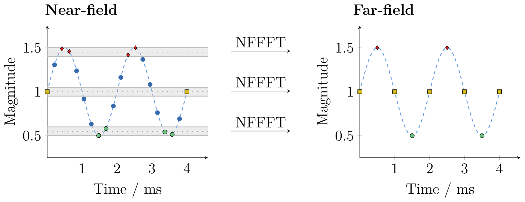
Figure 1Within the short-time measurement approach, field values which share the same modulation state can be transformed by the time-harmonic NFFFT. The signal can be directly reconstructed in the far field.
In fact, the constant modulation value mi might not be the same within one data set in reality as the exact value of mi depends on the specific sample times and also on the involved measurement uncertainties. Therefore, all values within an interval mi±ϵ are treated as equal as marked in Fig. 1. The short observation time of this STM makes the approach especially suitable for UAV-based antenna measurements since the error due to the movement of the UAV during data acquisition is kept small.
Measurements have been performed using a cylindrical NF measurement setup in an anechoic chamber at the Technical University of Munich. The double-ridged horn antenna DRH400 was employed as AUT and placed on a rotation table. Another horn antenna, HF906, served as field probe and was mounted 1.74 m away from the AUT on a vertical linear stage. The radius of the cylindrical measurement surface was equal to the distance between the antennas while the height of the cylinder was 1.5 m. Within all measurements, the AUT was transmitting and, therefore, connected to a signal generator of type R&S SMC100a which was set up to provide the requested amplitude or frequency modulation. A two-port vector network analyzer (VNA) of type R&S ZVK served as measurement receiver. However, it was only measuring two incoming b waves, where one channel was connected to the field probe and the other one to the signal generator feeding the AUT via a directional coupler. The additional measurement of the generator signal provides a phase reference to the receiver such that the complex field of the probe antenna can be measured. This non-classical measurement setup was chosen due to the fact that a reference signal will likely not be accessible in real in-situ measurement scenarios. In this case, a static reference antenna would be used to get the phase reference. The reference signal is also used for the classification of the measurement samples according to their modulation states mi and combining them into transformable data sets as described in Sect. 2. A schematic of the measurement setup is shown in Fig. 2.
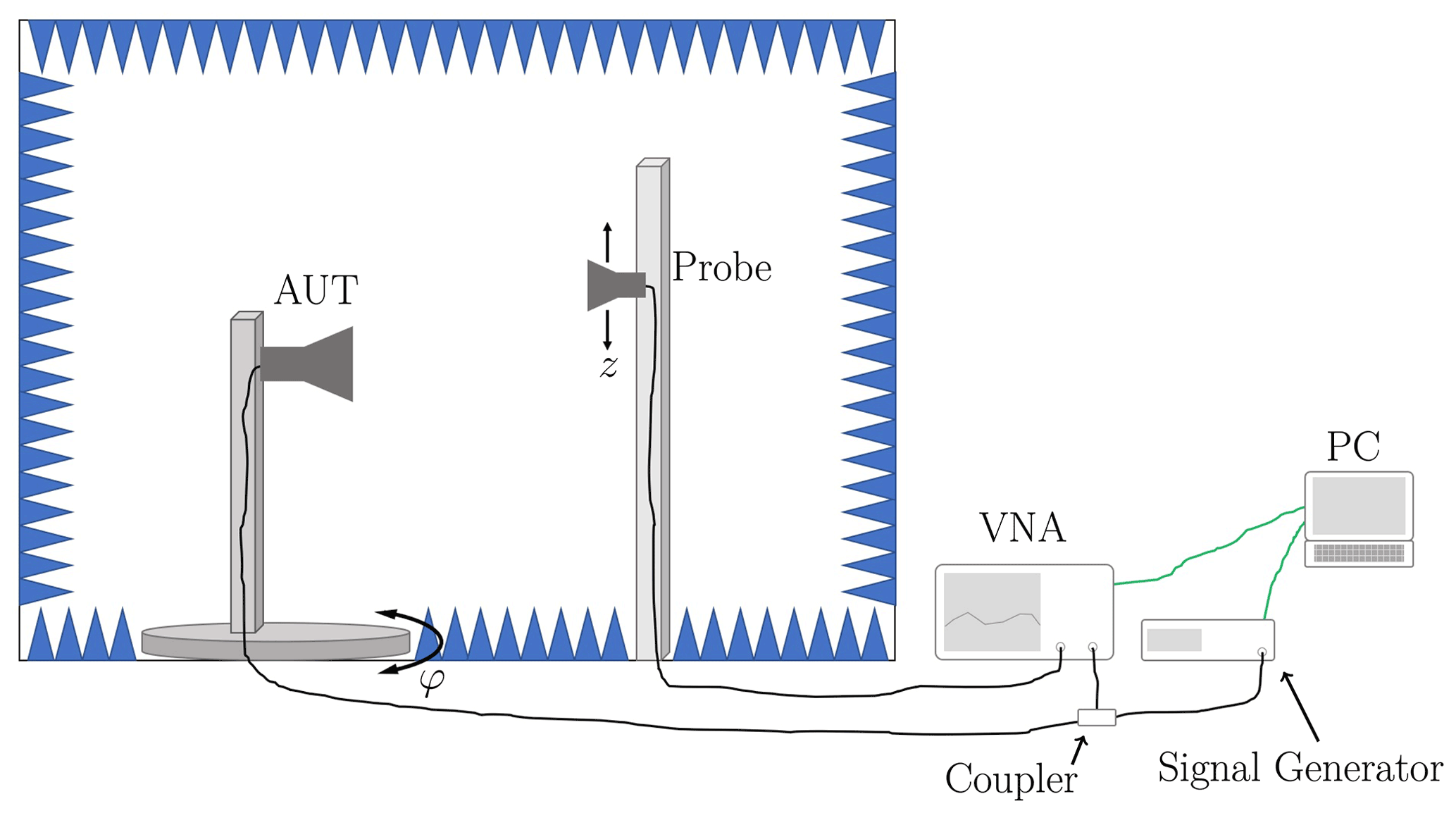
Figure 2The measurements have been performed in an anechoic chamber using a cylindrical antenna measurement setup. The AUT was mounted on a rotating table and the field probe on a vertical linear stage. A signal generator was used as source and a VNA as measurement receiver.
The usage of a VNA over, e.g., an oscilloscope, has the advantage that the large dynamic range, the good linearity, and all other benefits of a VNA are available in the setup. The VNA was measuring in zero-span mode, i.e., no frequency sweep was performed and all field samples were recorded at the carrier frequency. The zero-span mode has also the advantage that the sweep time depends only on the chosen measurement bandwidth, which, in addition, serves as an internal filter suppressing undesired noise outside the frequency range of interest, that may occur in in-situ measurement scenarios. As a result of several test measurements, the repeatability of the measurement setup was found to be −40 dB within the valid angles of the FF.
Step measurements have been performed in which the AUT and field probe are situated at fixed measurement locations during data acquisition. The carrier frequency was fc = 1 GHz and, first, an amplitude modulation (AM) with a frequency of fm=50 Hz and a modulation index of M=0.5 has been chosen. The measurement bandwidth was RBW = 3 kHz, which results in a measurement time of Tmeas = ms. The reference and measured NF signals in the main beam of the antenna are depicted in Fig. 3a.
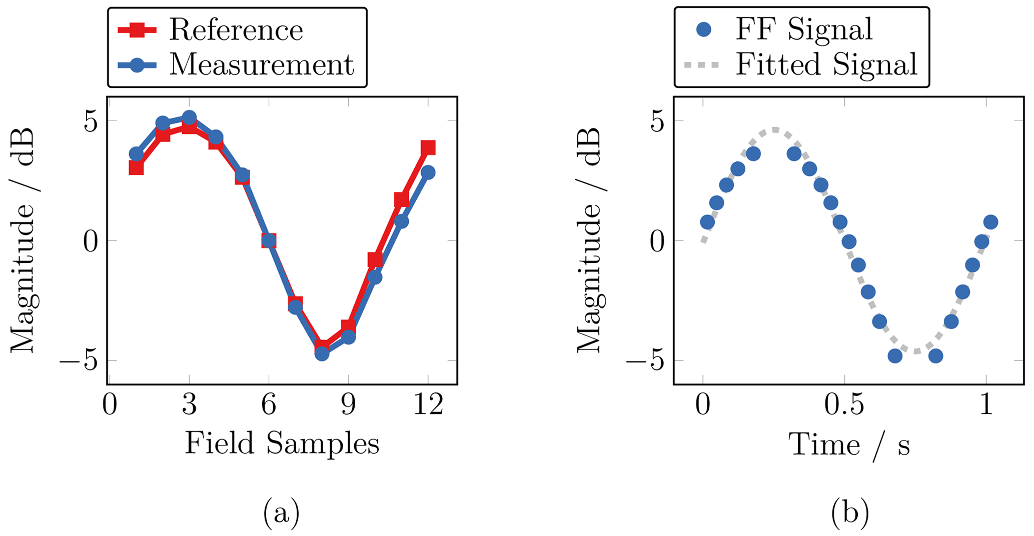
Figure 3Measured near-field signal in comparison to the reference (a) and corresponding far-field signal (b). The far-field signal has been reconstructed from the measured near field following the short-time measurement approach.
The corresponding FF signal in the main beam, i.e., ϑ = 90∘ and φ=0∘, is shown in Fig. 3b. The reconstruction of the FF signal depends on the actual filter process regarding the different modulation states mi and the pre-knowledge about the signal, e.g., whether it is symmetric or not.
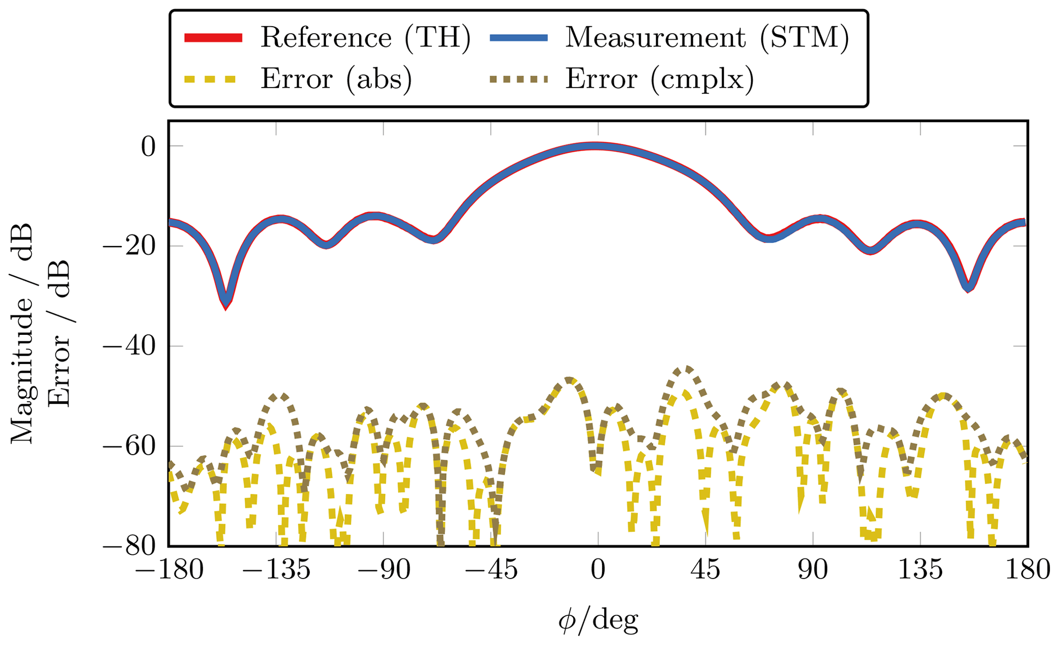
Figure 4Far-field main cut at ϑ=90∘. The deviation between the short-time measurement (STM) of the modulated field and the time-harmonic (TH) reference measurement is shown with (cmplx) and without (abs) the consideration of the phase of the field.
The FF main cut at ϑ=90∘ is depicted in Fig. 4. In the following, only the maximum error of this horizontal FF cut is shown for the maximum modulation state while other modulation states have been tested. Due to the cylinder height of only 1.5 m, the range within the valid angles is comparably small in vertical ϑ direction. This is only due to the measurement setup and has no limitations on the generality of the results, which has also been verified in simulations. The deviation between the modulated and the reference measurement is given by
and
where ESTM is the measured field and Eref the field obtained from a time-harmonic reference measurement. Often, FF measurement errors are calculated according to Eq. (4). However, Eq. (5) is more restrictive as the error measure includes magnitude and phase of the FF. Here, both error measures are shown to verify that the STM approach does not introduce additional phase errors into the measurements. Still, the more restrictive error according to Eq. (5) is for the majority of measurements slightly larger which is fully related to the measurement setup.
4.1 Amplitude modulation
To investigate the behavior of the STM approach for different modulation signals, first, the parameters of the amplitude modulation have been changed. According to the uncertainty principle in Eq. (2), the observation time is directly linked to the frequency resolution, which is similar to the resolution or measurement bandwidth (RBW) of the VNA. Figure 5a shows the maximum FF error for different RBWs.
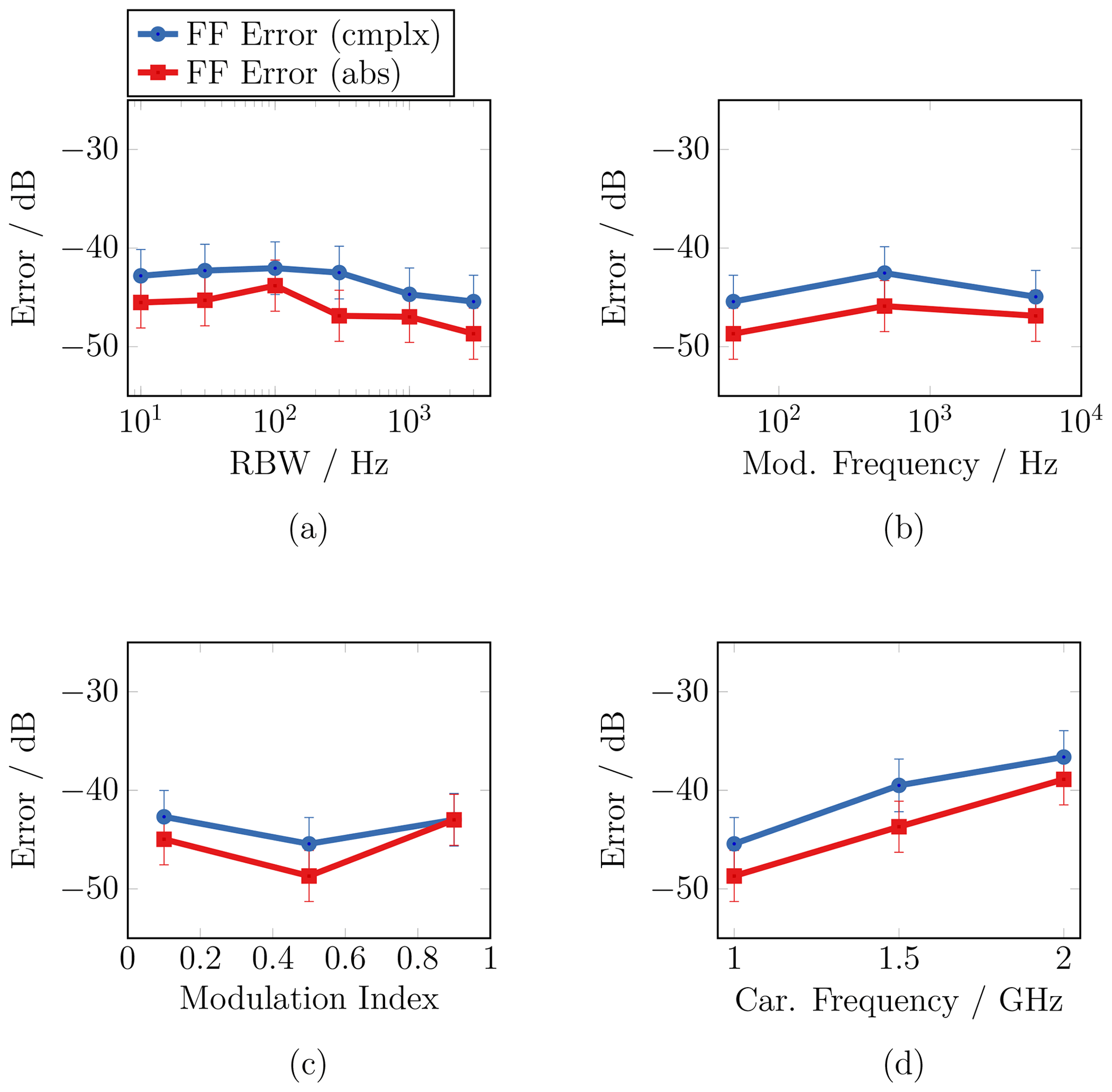
Figure 5Several step measurements have been performed where different signal parameters have been changed, such as the resolution bandwidth (a), the modulation frequency (b), the modulation index (c), and the carrier frequency (d). The absolute (red) and complex (blue) error measures are shown in comparison.
The measurements reveal that a longer observation time does not increase the FF error. Even a measurement time that is longer than the actual modulation period does not increase the transformation error. In this case, however, it is not possible to reconstruct the modulation signal in the FF as the modulation is simply averaged during the measurement. The change of the modulation frequency has a similar effect on the relation of the measurement time, respectively RBW, and the modulation period. The maximum error for different modulation frequencies in the range from 50 Hz to 5 kHz is depicted in Fig. 5b. Also here, no increase in the error can be observed when changing the modulation frequency. As stated before, the plots also reveal that the more restrictive FF error εcmplx is larger in the measurements in comparison to the absolute error εabs. Furthermore, the plot in Fig. 5c shows that the change of the index of the amplitude modulation has no significant impact on the maximum FF error. Nonetheless, it has to be mentioned that a large modulation index close to 1 can easily cause large errors for lower values of the modulation state, i.e., in or close to the minimum of the modulation signal, depending on the offset of the modulation, since the corresponding field values can be close to the noise floor of the measurement setup. In addition to the change of the parameters of the modulation signal, also the carrier frequency fc has been changed. The corresponding plot in Fig. 5d shows that the error increases for higher carrier frequencies. This is, however, not due to the STM approach as rather a consequence of the measurement setup. The used positioners have not been designed for NF measurements and do not share the high precision in positioning, which is necessary for NF measurements at higher frequencies. In contrast to the measurements, simulations show that the STM approach is independent of the actual carrier frequency.
4.2 Frequency modulation
Besides the measurements with an amplitude modulated signal, also measurements with a frequency modulation (FM) have been performed. Therefore, the internal input filter of the VNA has been used in such a way that an edge demodulation could be performed. This converts the initial FM to an AM and allows to process the measured field in the same way as described before. However, introducing an external filter right before the VNA could increase the accuracy of this FM-AM conversion as a linear frequency slope is required. The input filter of the VNA is undocumented and the best operation parameters have been, therefore, derived from several tests. The measurements with the FM were also performed at a carrier frequency of 1 GHz and a modulation frequency of 50 Hz. The frequency deviation was swept where the maximum FF error is depicted in Fig. 6.
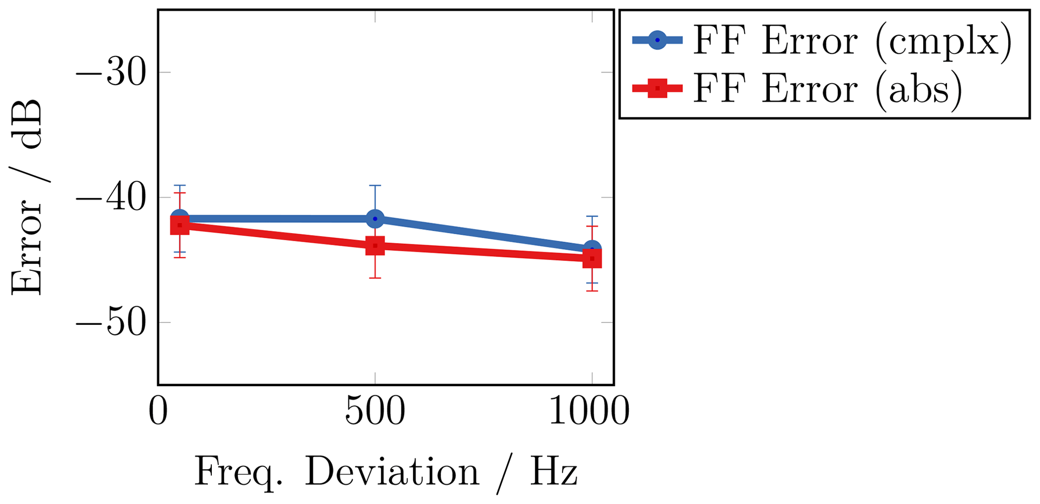
Figure 6Measurement error regarding a sweep of the frequency deviation for the case of a frequency modulated field.
The error level is comparable to the measurements in the AM case, while also no increase could be observed for the different frequency deviations.
As mentioned before, a UAV cannot hover at a specific position for a longer time, at least not with the high precision that is needed for NF measurements. Therefore, the case of a continuously flying UAV is considered, where, in the measurements, it has been emulated by the continuous movement of the field probe on horizontal lines of the cylindrical scan geometry. For this, the turntable was moving during all measurements with a constant angle velocity of vmove=12.4∘ s−1, which is equal to 0.375 m s−1 regarding the measurement distance in the setup. Again, measurements have been performed with an amplitude modulated field at a carrier frequency of 1 GHz. It is expected that the impact of the continuous UAV movement is increasing with longer observation times. Therefore, the RBW was chosen to 10 Hz, which results in an observation time of Tmeas=100 ms. Accordingly, the modulation frequency was chosen to 1 Hz and the modulation index to 0.5.
Figure 7a shows the maximum FF error for different modulation frequencies, while the error for different modulation indices is depicted in Fig. 7b.
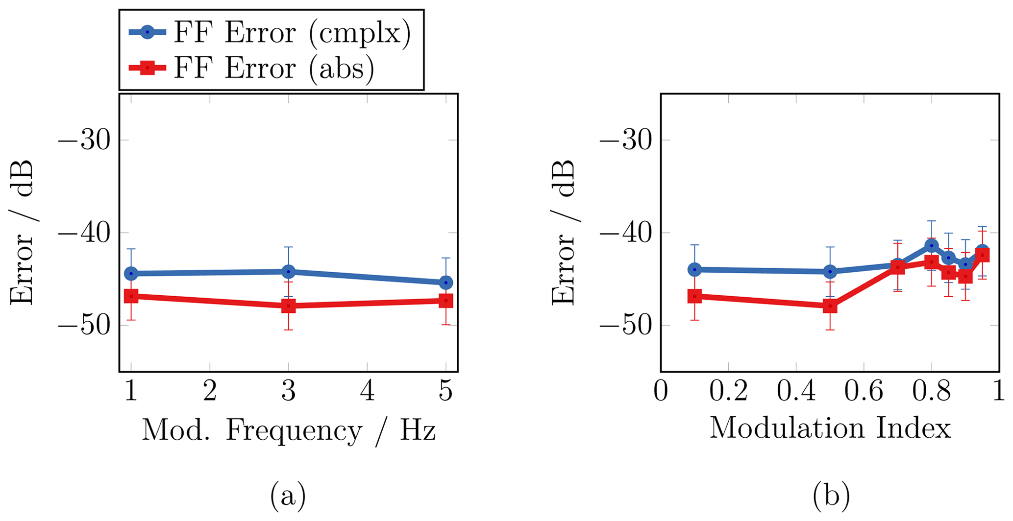
Figure 7The parameters of an amplitude modulated field have been swept for the case of a continuously moving field probe. The plots show the maximum far-field error for a sweep of the modulation frequency (a) and a sweep of the modulation index (b).
Both graphs reveal that, also in this case, the change of the measurement frequency as well as the modulation index does not lead to an increase in the FF error of the measurement. Despite these findings, it must be assumed that the ensemble of measurement time, modulation frequency, and movement velocity has an impact on the measurement of a modulated field. Therefore, further investigations of the limitation and error behavior of the STM approach have been performed with help of numerical simulations. The results have been published in Faul and Eibert (2021b). The simulations show that there are indeed configurations which cause a significant increase of the FF error. For example, it has been found that the FF error increases above a certain threshold frequency which mainly depends on the ensemble of measurement time and flight speed of the UAV. However, these configurations cannot be realized with the used measurement setup since neither measurement time Tmeas nor movement velocity vmove can be further increased. Nonetheless, the chosen relation of Tmeas and vmove in the presented measurements is realistic for real UAV-based NF measurements.
It has been shown that a short-time measurement approach can be applied to measure slowly continuously modulated field data. Measurements with amplitude and frequency modulated fields have been presented, where the field data was transformed to the far field by virtue of a time-harmonic NFFFT. Furthermore, two different cases have been considered: one where the field probe remains at static measurement locations during data acquisition and another one where the field probe is constantly moving on the cylindrical measurement surface such as a UAV would do in in-situ measurements. The different measurement results reveal that the short-time measurement approach does not cause a noticeable increase in the far-field error for the chosen parameter configurations, which are close to realistic in-situ measurement scenarios. Overall, the measurement results are in good agreement with numerical simulations, which have been published before.
The underlying research data can be requested from the authors.
FTF and TFE worked out the measurement concept. FTF and JD set up an appropriate measurement system and performed the measurements. JD evaluated the measurement data, supervised by FTF and TFE. All authors read and approved the final manuscript.
The contact author has declared that neither they nor their co-authors have any competing interests.
Publisher's note: Copernicus Publications remains neutral with regard to jurisdictional claims in published maps and institutional affiliations.
This article is part of the special issue “Kleinheubacher Berichte 2021”.
The authors thank Thomas Mittereder and Daniel Korthauer for their help during the measurements.
This research has been supported in part by the German Federal Ministry for Economic Affairs and Energy (grant no. 20E1711A).
This paper was edited by Romanus Dyczij-Edlinger and reviewed by two anonymous referees.
Eibert, T. F., Kilic, E., Lopez, C., Mauermayer, R. A. M., Neitz, O., and Schnattinger, G.: Electromagnetic field transformations for measurements and simulations (invited paper), Progress In Electromagnetics Research, 151, 127–150, 2015. a
Faul, F. T. and Eibert, T. F.: Setup and error analysis of a fully coherent UAV-based near-field measurement system, in: 15th European Conference on Antennas and Propagation (EuCAP), March 2021, Düsseldorf, Germany, 1–4, https://doi.org/10.23919/EuCAP51087.2021.9411307, 2021a. a
Faul, F. T. and Eibert, T. F.: Errors and prerequisites of the short-time measurement and transformation of continuously modulated fields, in: 43rd Antenna Measurement Techniques Association Symposium (AMTA), October 2021, Daytona Beach, Florida, USA, 1–6, https://doi.org/10.23919/AMTA52830.2021.9620725, 2021b. a
Faul, F. T., Kornprobst, J., Fritzel, T., Steiner, H.-J., Strauß, R., Weiß, A., Geise, R., and Eibert, T. F.: Near-field measurement of continuously modulated fields employing the time-harmonic near- to far-field transformation, Adv. Radio Sci., 17, 83–89, https://doi.org/10.5194/ars-17-83-2019, 2019. a
Faul, F. T., Steiner, H.-J., and Eibert, T. F.: Near-Field Antenna Measurements with Manual Collection of the Measurement Samples, Adv. Radio Sci., 18, 17–22, https://doi.org/10.5194/ars-18-17-2020, 2020. a
Faul, F. T., Daubmeier, J., and Eibert, T. F.: Short-time measurement and transformation of continuously modulated time-harmonic fields, in: Kleinheubacher Tagung, September 2021, Miltenberg, Germany, 1–4, https://doi.org/10.23919/IEEECONF54431.2021.9598410, 2021. a
Fernandez, M. G., Lopez, Y. A., and Andres, F. L.: On the use of unmanned aerial vehicles for antenna and coverage diagnostics in mobile networks, IEEE Commun. Mag., 56, 72–78, https://doi.org/10.1109/MCOM.2018.1700991, 2018. a
García-Fernández, M., Álvarez López, Y., Arboleya, A., González-Valdés, B., Rodríguez-Vaqueiro, Y., De Cos Gómez, M. E., and Las-Heras Andrés, F.: Antenna diagnostics and characterization using unmanned aerial vehicles, IEEE Access, 5, 23563–23575, https://doi.org/10.1109/ACCESS.2017.2754985, 2017. a
Geise, A., Neitz, O., Migl, J., Steiner, H.-J., Fritzel, T., Hunscher, C., and Eibert, T. F.: A crane based portable antenna measurement system – system description and validation, IEEE T. Antenn. Propag., 67, 3346–3357, https://doi.org/10.1109/TAP.2019.2900373, 2019. a
Hamberger, G. F., Corbett, R., and Derat, B.: Near-field techniques for millimeter-wave antenna array calibration, in: 40th Annual Symposium of the Antenna Measurement Techniques Association (AMTA), October 2019, San Diego, CA, 45–49, https://doi.org/10.23919/AMTAP.2019.8906415, 2019. a
Hansen, T. B. and Yaghjian, A. D.: Formulation of probe-corrected planar near-field scanning in the time domain, IEEE T. Antenn. Propag., 43, 569–584, https://doi.org/10.1109/8.387172, 1995. a
He, H., Maheshwari, P., and Pommerenke, D. J.: The development of an EM-field probing system for manual near-field scanning, IEEE T. Electromagn. C., 58, 356–363, https://doi.org/10.1109/TEMC.2015.2496376, 2016. a
Mauermayer, R. A. M. and Eibert, T. F.: Spherical field transformation above perfectly electrically conducting ground planes, IEEE T. Antenn. Propag., 66, 1465–1478, https://doi.org/10.1109/TAP.2018.2794406, 2018. a
Oetting, C.-C. and Klinkenbusch, L.: Near-to-far-field transformation by a time-domain spherical-multipole analysis, IEEE T. Antenn. Propag., 53, 2054–2063, https://doi.org/10.1109/TAP.2005.848465, 2005. a
Paonessa, F., Virone, G., Capello, E., Addamo, G., Peverini, O. A., Tascone, R., Bolli, P., Pupillo, G., Monari, J., Schiaffino, M., Perini, F., Rusticelli, S., Lingua, A. M., Piras, M., Aicardi, I., and Maschio, P.: VHF/UHF antenna pattern measurement with unmanned aerial vehicles, in: IEEE Metrology for Aerospace (MetroAeroSpace), https://doi.org/10.1109/MetroAeroSpace.2016.7573191, 87–91, 2016. a
Parini, C., Gregson, S., McCormick, J., Janse van Rensburg, D., and Eibert, T.: Theory and Practice of Modern Antenna Range Measurements, vol. 2, The Institution of Engineering and Technology, 2nd edn., 2020. a
Paris, D., Leach, W., and Joy, E.: Basic theory of probe-compensated near-field measurements, IEEE T. Antenn. Propag., 26, 373–379, https://doi.org/10.1109/TAP.1978.1141855, 1978. a
Schrader, T., Bredemeyer, J., Mihalachi, M., Ulm, D., Kleine-Ostmann, T., Stupperich, C., Sandmann, S., and Garbe, H.: High-resolution signal-in-space measurements of VHF omnidirectional ranges using UAS, Adv. Radio Sci., 17, 1–10, https://doi.org/10.5194/ars-17-1-2019, 2019. a
Sommer, D., Irigireddy, A. S. C. R., Parkhurst, J., Pepin, K., and Nastrucci, E. R.: UAV-based measuring system for terrestrial navigation and landing aid signals, in: AIAA/IEEE 39th Digital Avionics Systems Conference (DASC), October 2020, 1–7, https://doi.org/10.1109/DASC50938.2020.9256447, 2020. a
Yaghjian, A.: An overview of near-field antenna measurements, IEEE T. Antenn. Propag., 34, 30–45, https://doi.org/10.1109/tap.1986.1143727, 1986. a
Yinusa, K. A. and Eibert, T. F.: A multi-probe antenna measurement technique with echo suppression capability, IEEE T. Antenn. Propag., 61, 5008–5016, https://doi.org/10.1109/TAP.2013.2271495, 2013. a