Using Autoencoders to Classify EMC Problems in Electronic System Development

This paper is a direct continuation of “AI Assisted Interference Classification to Improve EMC Troubleshooting in Electronic System Development” (Maalouly et al., 2022). The previous paper aimed to classify the electromagnetic compatibility (EMC) problem classification, while this paper addresses two primary issues: the data and the technique. The technique used in the previous study involved a principal component analysis (PCA) (Pearson, 1901) to generate input features for the neural network. However, since PCA only encodes linear relations from the samples, autoencoder (AE) models are now used to encode the data into a latent vector that better represents the data. The latent vectors will ultimately be used as input to classify the EMC problems. A neural network and a random forest classifier were utilized to develop a classification model, wherein the random forest demonstrated superior performance in comparison to the neural network.

1 Introduction

Electromagnetic compatibility (EMC) problems are a significant concern in the printed circuit board (PCB) and chip design. The increase of electronic devices has brought these issues to the fore, with mobile phones, sensors, entertainment systems, and so forth now integral to everyday life. The manufacturing process of such devices is a complex and challenging undertaking. Consequently, the EMC issue is addressed during the design and development phase. However, identifying the source of the EMC problem is a difficult and resource-intensive task, which may prove particularly challenging for small and medium-sized enterprises. Therefore, a novel approach to identifying the source of EMC problems using elctromagnetic frequency spectra classification is studied and proposed. This study aims to detect these issues by using measurement spectra as input to an intelligent model for classification. However, the input data can become very large, which can cause the network to underperform. To address this issue, dimensionality reduction techniques are implemented to reduce the data complexity.

Eliardsson and Stenumgaard (2019) explores the use of AI, specifically machine learning, to automatically monitor and classify electromagnetic interference (EMI) in safety-critical wireless systems. It demonstrates how a k-nearest neighbors (k-NN) algorithm can identify interference signals in air-traffic control, highlighting AI's potential in Electromagnetic Compatibility (EMC) applications. Artificial intelligence has the potential to be utilized in multiple domains within the field of EMC. Zhang (2024) proposes a deep learning method to predict electromagnetic emission spectra in EMC tests of aerospace products. To enhance prediction accuracy while avoiding overfitting, a threshold-based data decomposition method is employed. A long short-term memory (LSTM) neural network is utilized, with hyperparameters optimized via Bayesian methods. This paper follows the previous work of Maalouly et al. (2022) where machine learning methods are employed to categorize distinct PCB layouts based on their electromagnetic frequency spectra, derived from simulated near-field measurements of electric fields. The training data, obtained by varying transmission line geometries, were transformed from the time domain to the frequency domain and utilized as input for a deep neural network. Principal component analysis reduced the data's dimensions. The results demonstrated high accuracy in classifying designs using synthetic data.

For now, the data required to train a classification model must be either real or possess characteristics similar to a real dataset. The data were generated by an electromagnetic field simulator. Due to the high computational effort, some additional physical optimizations are applied to the simulation models and current computational hardware with GPU acceleration is used in a parallel network. To further accelerate this and make it free from human errors in model generation, the simulation models are created, executed, and extracted in an automated way. The data are then parsed and treated to be used by the AE and later for the training of a classification neural network.

This paper begins with an overview of the real and simulated datasets. It then proceeds to describe the pipeline, beginning with data processing and continuing with the autoencoder networks. This is followed by an examination of the use of reduced data with a classification neural network and a random forest classifier. The paper concludes with a presentation of the results and a discussion of the conclusions.

2 Dataset

2.1 Real Data

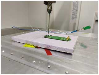
The training data are generated using a hybrid approach of real EMC near and farfield measurements and electromagnetic field simulation based on the same PCB basic layout. In general, the hardware setup contains differential pair transmission lines, which are excited by a frequency adjustable (clock) signal generator. The variation parameters are chosen to be the ground (GND) plane geometry below the transmission lines, their line impedance, the termination impedance as far as the dimensioning of decoupling capacitors in the power delivery network (PDN). The parameter variations were coarse-stepped for the real measurements and finer resolutions are used for the simulations in order to achieve a sufficient amount of training data. In order to allow for some simplifications in simulation model complexity, radiated emission measurements in a semi-anechoic chamber based on test setups according to EN 55011 were carried out to obtain real datasets which can be extended by simulation. The PCBs were placed on a non-conductive table (ε_r≈1.2) with a height of 80 cm above the conductive ground plane. The phase-centre of the measurement antenna is placed in a distance of 3 m from the centre of the PCB. Measurements were carried out in the frequency range 30 to 1000 MHz using a bandwidth of 120 kHz with peak and average detection. By the measurement of 30 hardware samples using two excitation frequencies and two wire lengths (300, 2000 mm) for the power supply, a total number of 1440 data samples are generated. However, as the emission is generated by a narrowband disturbance source, the peak and average detection results are highly correlated, which has to be taken into account. Another way to obtain real measurement data for the radiation is to use near-field scans. The electric and magnetic field components (x, y & z) are measured using near-field probes. These measurements are taken at various locations around the DUT (device under test) (Claeys, 2018). The near-field scanner NFS3000 from Fraunhofer ENAS in Paderborn, Germany was used as the measuring instrument (Schroeder et al., 2020). Figure 1 shows a photo of this near-field measurement. The probe above the DUT measures the respective signal strength (here: H_t) and the exposed conductor loop on the right is used as a reference signal for calculating the phase. The results of these magnetic tangential field measurements are represented in Fig. 2. Here, the PCB was excited with a 50 MHz square wave signal on channel 1 and shows the main signal and the first two harmonics, respectively. The representation of the tangential electric and magnetic fields around a closed surface can be used as an equivalent source using the Surface Equivalence Principle or the BEM (Boundary Element Method) (Sievers, 2008). These substitute sources can then be used for a far-field transformation. The mathematical principles and conditions are described in Lange et al. (2020) and Marschalt et al. (2022). The result of this near-field to far-field transformation (NF2FF) is shown in Fig. 3.

Figure 1 DUT during near-field measurement.

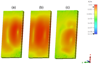
Figure 2 Maximum tangential magnetic field strengths of the PBC board, which was excited with a 50 MHz square wave signal, as a replacement source for an NF2FF. (a) 50 MHz, (b) 150 MHz, (c) 250 MHz.

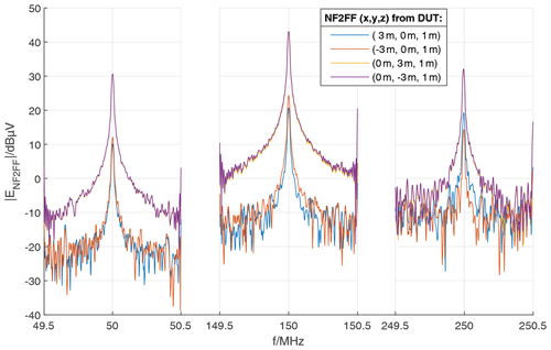
Figure 3 NF2FF Results from the near-field measurement on the PCB at various spatial coordinates, which was excited with a 50 MHz square-wave signal.

This means that the near-field data can then be used in the same way as the far-field measurements by the NF2FF, although a completely different measurement method was used.

2.2 Simulation Data

As measurements are very time-consuming and many variants are required for the training data, which would also be very cost-intensive, the necessary training data are complemented by simulations. For this purpose, the circuit board from Fig. 1 was modeled as a simulation model, which was also excited at f=50 MHz on channel 1 in Fig. 4. Here it is much easier to generate the necessary variants for the different training data.

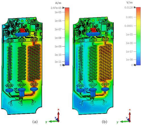
Figure 4 Maximum magnetic (a) and electric (b) field distributions on the simulation model of the PCB with an activated 50 MHz square wave signal on the right trace (channel 1).

In order to obtain very realistic results, the Finite Integration Technique (FIT) (Weiland, 1977) was used here in the time domain, as this allows very broadband results to be used in a simulation as well as real signal shapes. In order to adapt the radiation behavior to the real environment of an anechoic chamber with a steel floor, corresponding boundary conditions were defined in the simulation and not the complete measurement environment was modeled, as this would increase the calculation time enormously. Instead of the absorber structures PML (perfectly matched layer) (Berenger, 1994) and a PEC (Perfect Electrical Conductor) (Lindell and Sihvola, 2005) boundary condition was selected for the steel floor. To save further calculation time, an NF2FF was also used here by simulating only the size around the table required by convergence studies and calculating the rest using the NF2FF (Gibson, 2008). These adjustments can be seen in Fig. 5.

Figure 5 Reduction of the simulation volume and the resulting simulation time by using the NF2FF.

These adjustments have already enabled highly complex simulation models to be created for more than 80 000 training data pairs with variations of the DUT as input parameters and radiation behavior as far-field spectra. The variations differed in the form of transmission lines, GND structure, various additional impedances (at short-circuit and load resistors) and signal types. The simulated data are then parsed between two different classes. The first class is the termination [good, bad] while the second is the frequency [50 MHz, 100 MHz]. All simulated data assumes a line impedance value of 100 Ω. A termination is considered good if its resistance aligns with the line impedance of 100 Ω within a tolerance of ±15 %. Termination resistance ranging from 85 to 115 Ω is considered optimal, while values outside this range are considered suboptimal.

3 Classification Model

3.1 Pipeline

The pipeline processes raw data and converts it into a readable format for our models. The selected frequency classes are between 50 and 100 MHz, and the termination is either good or bad. The data labels are parsed to meet the requirements to start the encoding process using an AE model. Once the AE model is constructed, the data are encoded into the desired number of latent dimensions to extract the necessary features. The neural networks described in the following sections are constructed using Python and TensorFlow (Abadi et al., 2015), while the random forest classifier is constructed using Scikit-learn (Pedregosa et al., 2011).

3.2 Autoencoder

An AE is a type of unsupervised neural network. It consist of two networks, an encoder, and a decoder, working together to learn an efficient representation of input data. The main purpose of autoencoders is to encode input data into a lower-dimensional (latent dimension) representation and then decode it back to reconstruct the original input. The advantage of using an AE network is the learning of the latent dimension in a non-linear fashion in contrast to a principle component analysis, which is only capable of capturing linear relations.

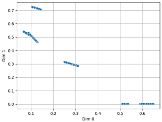
The data collected and parsed have totaled to 353 samples. Each sample contains 1001 farfield measurements from frequencies ranging between [30 MHz–1000 MHz]. The frequency classes are properly distributed while the termination class holds a slight imbalance. The latent dimensions (l) chosen are l=2 and l=200. The reduction to l=2 allows for the visualization of the dataset and to check if any clustering exists. The data are reduced from 1001 dimensions to 2 dimensions. Figure 6 is a visualization of the simulated data showing a typical behavior for a simulation where the sample points are almost linear in structure. Clustering is also visible within the simulated dataset.

Figure 6 Encoding the simulated data using the AE model.

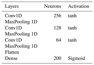
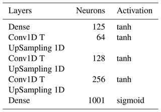
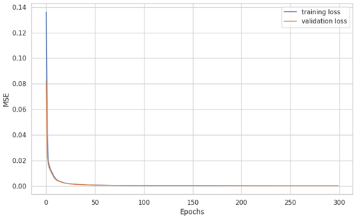
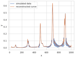
As the latent dimension increases the information loss will be less and less severe. Tables 1 and 2 shows the encoder and decoder network architectures respectively. The latent dimension chosen is of size 200 for the training of the classification neural network. The training is done over 300 epochs with a batch size of 256. Adam optimizer is used along with a 0.0001 learning rate with a mean squared error as a loss function. The model achieved a low loss error as seen in Fig. 7 meaning the model learned to encode the data efficiently with minimum information loss. The reconstruction of a simulated measurement curve should ideally resemble the initial input curve as in Fig. 8. The data are then run into the encoder to reduce the data dimensionality. The result is a dataset of size [352, 200] and a corresponding label set of [352, 3].

Table 1 The encoder network architecture.

Table 2 The decoder network architecture.

Figure 7 The training loss function for the AE.

Figure 8 Simulated data measurement sample and its reconstruction.

3.3 Classification Network

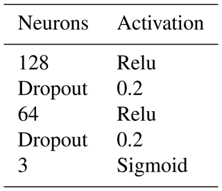
With the data now reduced, the training of the classification neural network can start. The classification network takes an input of 200 features and outputs the predicted classes. The network uses an Adam optimizer with a learning rate of 0.0001 and a batch size of 32. The data is split into training and testing sets with the latter being 10 % of the dataset. Furthermore, the training data are then split into 2 sets, one for training and the other for validation being 20 % of the training data. Since this is a multiclass problem the loss used is the Binary Crossentropy with 300 training epochs with Table 3 showing the network architecture.

Table 3 The classification network architecture.

3.4 Classification Network Results

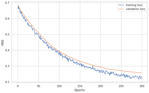
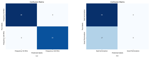
The network achieved a low training and validation loss of approximately 0.2, with slight indications of overfitting, as demonstrated in Fig. 9. This suggests that the model has difficulty distinguishing between one of the classes. To further analyze this, the confusion matrix of Fig. 10 is examined. The frequency classes are perfectly discriminated, which is a very predictable behavior due to the high correlation between the feature set and the frequency classes (Maalouly et al., 2024). However, there is no correlation between the termination and the feature set, but rather a clustering behavior. The unbalanced number of samples in the Good Termination class coupled with the number of total samples resulted in an overfit model specifically for identifying the termination class. A solution would be to reduce the complexity of the model to better identify the clusters.

Figure 9 Classification loss function.

Figure 10 Frequency confusion matrix (a) and termination confusion matrix (b) from the classification neural network.

3.5 Random Forest

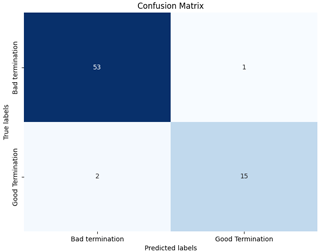
Random Forest is a machine learning algorithm used for both classification and regression tasks (Ho, 1995). It is an ensemble learning technique that combines multiple models to improve their predictive capabilities. During the training phase, a Random Forest creates a multitude of decision trees. The performance of a model can be improved or weakened by the number of trees selected. To construct each decision tree, a random subset of features from the training data are selected and decisions are made based on those features. In the previous section, the sample data could not be classified by the network according to their respective termination. That is due to low the correlation to the output class and the bias in the dataset. Therefore, a machine learning model is better equipped to handle such problems. Random forest was applied with different tree values as a hyperparameter. Using 10 tree estimators resulted in the highest accuracy, with a training accuracy of 0.996 and a test accuracy of 0.957. Figure 11 shows the resulting confusion matrix for the termination.

Figure 11 The confusion matrix using the test data with random forest classification.

4 Conclusions

In this paper, a hybrid data generation approach is taken to better validate the authenticity of the simulated data. The simulated data are first parsed to a readable format, fit for the consumption of the networks. Then, an AE network is constructed to take in the simulated data and output an encoded form. As a next step, the encoded data are passed along to the classification neural network for the detection of the output classes termination [Good, Bad] and frequency [50 MHz, 100 MHz]. The classification network shows the ability to classify the frequency class reliably, however, the aid of a random forest classifier is needed for the classification of the termination. It can be reasonably deduced that the measurement spectra allow for the extraction of certain key features that can be used to identify specific EMC problems. However, the extent to which this is possible has yet to be tested. For the next steps, the aim is to add more classes however, the more classes are added the more complex the problem becomes. Another task would be to bridge the gap between real and simulated data. Although, a hybrid approach is used the model still needs to be tested on real data.