A Numerical Alternative for 3D Addition Theorems Based on the Bilinear Form of the Dyadic Green's Function and the Equivalence Principle

A numerical method based on the equivalence principle and the dyadic Green's function is presented. It can be used to compute the spherical-multipole amplitudes with respect to an origin in a subdomain 2 due to sources in a distinct subdomain 1. As an example, consider that subdomain 1 contains a horn antenna that is solved numerically using a commercial full-wave simulator. The radiated field serves as the incident field for subdomain 2 which contains the scatterer, in our example a lossless dielectric sphere. The proposed method is based on the equivalence currents on a Huygens surface enclosing the antenna and uses the free-space dyadic Green's function to compute the electric and magnetic fields on a sphere enclosing the scatterer. From this electromagnetic field on the spherical surface, the spherical-multipole amplitudes of the incident field with respect to the center of the sphere enclosing the scatterer are obtained numerically and can be further processed. The results obtained with this method are compared to the results solely computed by the numerical full-wave simulator.

1 Introduction

Computational Electromagnetics plays a crucial role in electrical engineering, with many applications in microwave techniques, antennas, and propagation, among others (Davidson, 2010; Sumithra and Thiripurasundari, 2017). Several methods have been developed to solve electrically large problems, where the typical size of the structure exceeds tens or even hundreds of wavelengths. In this context, the case of objects separated by a homogeneous background medium is of particular interest and will be addressed in the following.

A typical approach to solving such problems is based on a physical domain decomposition, that is, to first solve the electromagnetic problem in each of the subdomains separately and to subsequently find the solution of the entire problem by letting the subdomain solutions interact through a suitable coupling procedure. The electromagnetic problem in each of the subdomains and the coupling can be solved by a specialized numerical method.

An example for a related method can be found in a recent work by Losenicky et al. (2021), where the Method of Moments (MoM) and the T-matrix approach are combined. In particular, there the MoM is used to solve the radiator, an electric dipole, and the fields are projected on a sphere enclosing the radiator to obtain a multipole representation. This is then used to translate the multipoles and solve the scattering problem in another subdomain. However, this approach requires that the subdomains are enclosed by two non-intersecting spheres; therefore, this method does not allow having the antenna and the scatterer in close proximity. This aspect is more limiting when the aspect ratio of the antenna or the scatterer is large, e.g., an electric dipole which is large in one dimension and small in the other two. Other instances of related approaches are found in Alian and Oraizi (2018, 2019), where the addition theorem is combined with the equivalence principle algorithm (EPA) (Li et al., 2006; Li and Chew, 2007) to solve scattering problems with multiple PEC objects. Again, spheres enclosing the objects which must not intersect are needed to apply the method. Additionally, in Alian and Oraizi (2018, 2019) far fields are analyzed; hence no radiator is included in the analysis.

In the present work, we extend the 2D multipole approach we introduced in Giannetti and Klinkenbusch (2023) to the 3D case. The method is based on the equivalence principle and the free-space dyadic Green's function. Two subdomains are considered: one contains an antenna, and the other a scatterer. The classical approach is based on the addition theorem for vector spherical-multipole functions (VSMFs) and requires the Huygens surface enclosing the radiator to be a sphere. The method described here allows one to enclose the radiator with a Huygens surface of arbitrary shape. Hence, it is more flexible and the distances between the different subdomains can be reduced. The field radiated by the scatterer can then be computed using a spherical-multipole expansion centered at subdomain 2 and a suitable solver​​​​​​​. The scatterer can have an arbitrary geometry – though the analysis naturally simplifies for a spherical scatterer, e.g. the model of the human head as used in Losenicky et al. (2021).

The paper is organized as follows. The problem is outlined in Sect. 2 while the proposed method is described in Sect. 3. First numerical results and some conclusions are shown in Sects. 4 and 5, respectively.

2 Formulation of the Problem

Figure 1 shows the problem and the used notations. The scatterer is enclosed by a spherical surface of radius R_s. In the phasor domain and at a time factor e^+jωt, the total field for $r^{\prime }\ge R_{\mathrm{s}}$ is split into an incident and a scattered part. The multipole expansions of the corresponding electrical fields are given by (Klinkenbusch, 2008)

$$\begin{array}{}\text{(1)}& {\displaystyle }{\mathit{E}}^{\mathrm{i}}\left({\mathit{r}}^{\prime }\right)=\sum _{n,m}{a}_{n,m}^{\mathrm{i}}{\mathit{N}}_{n,m}^{\left(\mathrm{1}\right)}\left({\mathit{r}}^{\prime }\right)+{\displaystyle \frac{Z}{j}}\sum _{n,m}{b}_{n,m}^{\mathrm{i}}{\mathit{M}}_{n,m}^{\left(\mathrm{1}\right)}\left({\mathit{r}}^{\prime }\right)\text{(2)}& {\displaystyle }{\mathit{E}}^{\mathrm{s}}\left({\mathit{r}}^{\prime }\right)=\sum _{n,m}{a}_{n,m}^{\mathrm{s}}{\mathit{N}}_{n,m}^{\left(\mathrm{2}\right)}\left({\mathit{r}}^{\prime }\right)+{\displaystyle \frac{Z}{j}}\sum _{n,m}{b}_{n,m}^{\mathrm{s}}{\mathit{M}}_{n,m}^{\left(\mathrm{2}\right)}\left({\mathit{r}}^{\prime }\right),\end{array}$$

respectively. Here, $Z=\sqrt{\mathit{\mu }/\mathit{\epsilon }}$ is the intrinsic wave impedance of the medium (vacuum is considered in the following) and ${\sum }_{n,m}={\sum }_{n=\mathrm{1}}^N{\sum }_{m=-n}^n$, $a_{n,m}^{\mathrm{i}\left(\mathrm{s}\right)}$ and $b_{n,m}^{\mathrm{i}\left(\mathrm{s}\right)}$ represent the multipole coefficients of the incident and scattered electromagnetic fields, respectively. The vector spherical-multipole functions (VSMF) ${\mathit{N}}_{n,m}^{\left(q\right)}\left(\mathit{r}\right)$ and ${\mathit{M}}_{n,m}^{\left(q\right)}\left(\mathit{r}\right)$ are defined by (Klinkenbusch, 2008)

$$\begin{array}{}\text{(3)}& {\displaystyle }{\mathit{M}}_{n,m}^{\left(q\right)}\left(\mathit{r}\right)=z_n^{\left(q\right)}\left(kr\right){\mathit{m}}_{n,m}(\mathit{\theta },\mathit{\varphi })\text{(4)}& {\displaystyle }\begin{array}{rl}{\mathit{N}}_{n,m}^{\left(q\right)}\left(\mathit{r}\right)=& -{\displaystyle \frac{z_n^{\left(q\right)}\left(kr\right)}{kr}}n(n+\mathrm{1})Y_{n,m}(\mathit{\theta },\mathit{\varphi })\widehat{r}\\ & +w_n^{\left(q\right)}\left(kr\right){\mathit{n}}_{n,m}(\mathit{\theta },\mathit{\varphi }).\end{array}\end{array}$$

Here, $w_n^{\left(q\right)}\left(kr\right)=-\frac{\mathrm{1}}{kr}\frac{\mathrm{d}}{\mathrm{d}r}\left(r{z}_n^{\left(q\right)}\left(kr\right)\right)$, $\widehat{r}$ is the unit vector in the radial direction, and $k=\mathit{\omega }\sqrt{\mathit{\epsilon }\mathit{\mu }}$ is the wavenumber of the homogeneous medium. The superscripts used here, (q)=(1) and (q)=(2), indicate that the radial dependence is given by spherical Bessel functions of the first kind ($z_n^{\left(\mathrm{1}\right)}=j_n$) or by spherical Hankel functions of the second kind ($z_n^{\left(\mathrm{2}\right)}=h_n^{\left(\mathrm{2}\right)}$), respectively. Note that spherical Bessel functions of the first kind are regular everywhere and must be used to represent regular fields at the origin (r=0), while at the given time factor only Hankel functions of the second kind comply with the radiation condition for r→∞.

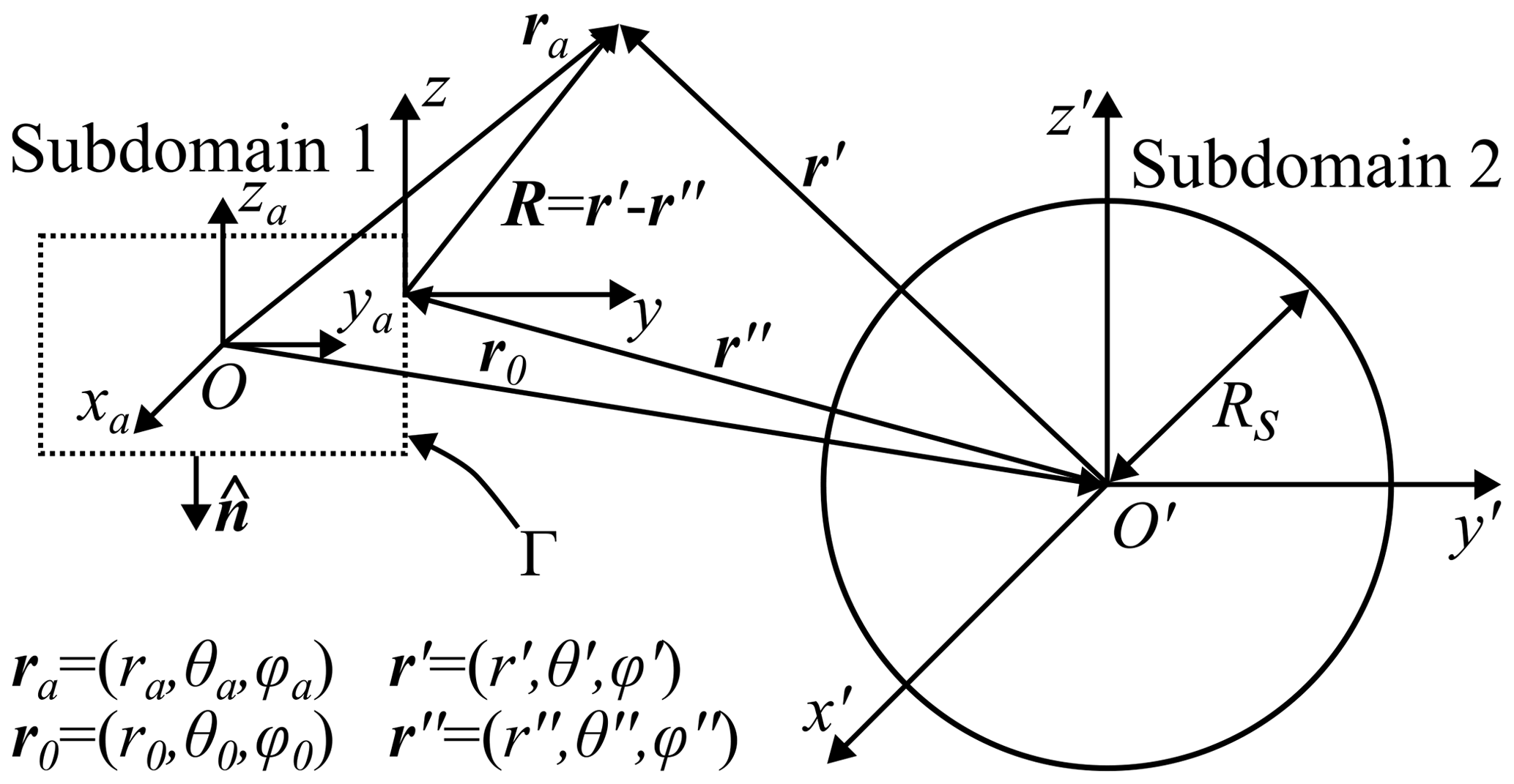
Figure 1 Definition of the problem: subdomain 1 (antenna), subdomain 2 (scatterer), and corresponding notations.

The transverse spherical multipole functions (TSMFs) ${\mathit{m}}_{n,m}(\mathit{\theta },\mathit{\varphi })$ and ${\mathit{n}}_{n,m}(\mathit{\theta },\mathit{\varphi })$ are defined as

$$\begin{array}{}\text{(5)}& {\displaystyle }{\mathit{m}}_{n,m}(\mathit{\theta },\mathit{\varphi })=-{\displaystyle \frac{\mathrm{1}}{\sin \left(\mathit{\theta }\right)}}{\displaystyle \frac{\partial Y_{n,m}(\mathit{\theta },\mathit{\varphi })}{\partial \mathit{\varphi }}}\widehat{\mathit{\theta }}+{\displaystyle \frac{\partial Y_{n,m}(\mathit{\theta },\mathit{\varphi })}{\partial \mathit{\theta }}}\widehat{\mathit{\varphi }}\text{(6)}& {\displaystyle }{\mathit{n}}_{n,m}(\mathit{\theta },\mathit{\varphi })={\displaystyle \frac{\partial Y_{n,m}(\mathit{\theta },\mathit{\varphi })}{\partial \mathit{\theta }}}\widehat{\mathit{\theta }}+{\displaystyle \frac{\mathrm{1}}{\sin \left(\mathit{\theta }\right)}}{\displaystyle \frac{\partial Y_{n,m}(\mathit{\theta },\mathit{\varphi })}{\partial \mathit{\varphi }}}\widehat{\mathit{\varphi }},\end{array}$$

where $\widehat{\mathit{\theta }}$ and $\widehat{\mathit{\varphi }}$ are the unit vectors along θ and ϕ, respectively, and where the surface spherical harmonics $Y_{n,m}(\mathit{\theta },\mathit{\varphi })$ are defined by

$$\begin{array}{}\text{(7)}& Y_{n,m}(\mathit{\theta },\mathit{\varphi })=\sqrt{{\displaystyle \frac{(n-m)\mathrm{!}}{(n+m)\mathrm{!}}}{\displaystyle \frac{\mathrm{2}n+\mathrm{1}}{\mathrm{4}\mathit{\pi }}}}{P}_n^m\left(\cos \right(\mathit{\theta }\left)\right)e^{jm\mathit{\varphi }}.\end{array}$$

Here, $P_n^m\left(\cos \right(\mathit{\theta }\left)\right)$ denotes an associated Legendre function of the first kind. Note that $Y_{n,-m}(\mathit{\theta },\mathit{\varphi })=(-\mathrm{1}{)}^m{Y}_{n,m}^{\ast }(\mathit{\theta },\mathit{\varphi })$ holds, with the asterisk indicating the complex conjugate.

In the absence of a scatterer, the scattered field vanishes and the total field is identical to the incident field, which is in this case also valid for r<R_s.

In case a scatterer is present, the multipole coefficients of the incident and scattered fields are related by the scattering matrix, which fully characterizes the scatterer. For the simple case of a homogeneous isotropic dielectric sphere with wavenumber k_s and intrinsic wave impedance Z_s, the scattering matrix is diagonal, and the relations between the multipole coefficients of the scattered and incident fields are found as

$$\begin{array}{}\text{(8)}& \begin{array}{rl}{\displaystyle \frac{a_{n,m}^{\mathrm{s}}}{a_{n,m}^{\mathrm{i}}}}& =-{\displaystyle \frac{b_{n,m}^{\mathrm{s}}}{b_{n,m}^{\mathrm{i}}}}\\ & ={\displaystyle \frac{w_n^{\left(\mathrm{1}\right)}\left(k{R}_{\mathrm{s}}\right)j_n\left(k_{\mathrm{s}}{R}_{\mathrm{s}}\right)-\frac{Z}{Z_{\mathrm{s}}}{w}_n^{\left(\mathrm{1}\right)}\left(k_{\mathrm{s}}{R}_{\mathrm{s}}\right)j_n\left(k{R}_{\mathrm{s}}\right)}{w_n^{\left(\mathrm{2}\right)}\left(k{R}_{\mathrm{s}}\right)j_n\left(k_{\mathrm{s}}{R}_{\mathrm{s}}\right)-\frac{Z}{Z_{\mathrm{s}}}{w}_n^{\left(\mathrm{1}\right)}\left(k_{\mathrm{s}}{R}_{\mathrm{s}}\right)j_n\left(k{R}_{\mathrm{s}}\right)}}.\end{array}\end{array}$$

Moreover, the field inside the dielectric sphere can be expanded using the spherical-multipole expansion

$$\begin{array}{}\text{(9)}& {\mathit{E}}^{\mathrm{in}}\left({\mathit{r}}^{\prime }\right)=\sum _{n,m}{a}_{n,m}^{\mathrm{in}}{\mathit{N}}_{n,m}^{\left(\mathrm{1}\right)}\left({\mathit{r}}^{\prime }\right)+{\displaystyle \frac{Z_{\mathrm{s}}}{j}}\sum _{n,m}{b}_{n,m}^{\mathrm{in}}{\mathit{M}}_{n,m}^{\left(\mathrm{1}\right)}\left({\mathit{r}}^{\prime }\right),\end{array}$$

with the multipole amplitudes

$$\begin{array}{}\text{(10)}& \begin{array}{rl}& a_{n,m}^{\mathrm{in}}={\displaystyle \frac{Z_{\mathrm{s}}}{Z}}{\displaystyle \frac{a_{n,m}^{\mathrm{i}}{j}_n\left(k{R}_{\mathrm{s}}\right)+a_{n,m}^{\mathrm{s}}{h}_n^{\left(\mathrm{2}\right)}\left(k{R}_{\mathrm{s}}\right)}{j_n\left(k_{\mathrm{s}}{R}_{\mathrm{s}}\right)}}\\ & b_{n,m}^{\mathrm{in}}={\displaystyle \frac{b_{n,m}^{\mathrm{i}}{w}_n^{\left(\mathrm{1}\right)}\left(k{R}_{\mathrm{s}}\right)+b_{n,m}^{\mathrm{s}}{w}_n^{\left(\mathrm{2}\right)}\left(k{R}_{\mathrm{s}}\right)}{w_n^{\left(\mathrm{1}\right)}\left(k_{\mathrm{s}}{R}_{\mathrm{s}}\right)}}.\end{array}\end{array}$$

3 Proposed method

First, we apply the equivalence principle with a Huygens surface that completely encloses the antenna (Fig. 1). There, the equivalent currents, that completely represent the antenna outside its subdomain, are given by (Balanis, 2012)​​​​​​​

$$\begin{array}{}\text{(11)}& {\mathit{J}}_{\mathrm{eq}}=\widehat{\mathit{n}}\times {\mathit{H}}^a\left(\mathrm{\Gamma }\right),{\mathit{M}}_{\mathrm{eq}}=-\widehat{\mathit{n}}\times {\mathit{E}}^a\left(\mathrm{\Gamma }\right),\end{array}$$

where Γ is the Huygens surface, and $\widehat{\mathit{n}}$ the unit vector directed outwards (Fig. 1). The equivalent currents Eq. (11) are calculated from the fields delivered by a full-wave simulator.

The electromagnetic field outside of the Huygens surface can be expressed with respect to the coordinate system of subdomain 2 according to (Li et al., 2006; Alvarez et al., 2007; Quijano et al., 2011; Balanis, 2012)

$$\begin{array}{}\text{(12)}& {\displaystyle }\mathit{E}\left({\mathit{r}}^{\prime }\right)=-jkZ\mathcal{L}\left({\mathit{J}}_{\mathrm{eq}}\left({\mathit{r}}^{\prime \prime }\right)\right)-\mathcal{K}\left({\mathit{M}}_{\mathrm{eq}}\left({\mathit{r}}^{\prime \prime }\right)\right)\text{(13)}& {\displaystyle }\mathit{H}\left({\mathit{r}}^{\prime }\right)=-jkY\mathcal{L}\left({\mathit{M}}_{\mathrm{eq}}\left({\mathit{r}}^{\prime \prime }\right)\right)+\mathcal{K}\left({\mathit{J}}_{\mathrm{eq}}\left({\mathit{r}}^{\prime \prime }\right)\right),\end{array}$$

where the integral operators 𝒦 and ℒ are defined by

$$\begin{array}{}\text{(14)}& {\displaystyle }\mathcal{K}\left({\mathit{I}}_{\mathrm{eq}}\left({\mathit{r}}^{\prime \prime }\right)\right)=\underset{\mathrm{\Gamma }}{\int }{\mathrm{\nabla }}^{\prime }g({\mathit{r}}^{\prime },{\mathit{r}}^{\prime \prime })\times {\mathit{I}}_{\mathrm{eq}}\left({\mathit{r}}^{\prime \prime }\right)\mathrm{d}{S}^{\prime \prime }\text{(15)}& {\displaystyle }\mathcal{L}\left({\mathit{I}}_{\mathrm{eq}}\left({\mathit{r}}^{\prime \prime }\right)\right)=\underset{\mathrm{\Gamma }}{\int }\stackrel{\mathrm{‾}}{\stackrel{\mathrm{‾}}{G}}\left({\mathit{r}}^{\prime },{\mathit{r}}^{\prime \prime }\right)\cdot {\mathit{I}}_{\mathrm{eq}}\left({\mathit{r}}^{\prime \prime }\right)\mathrm{d}{S}^{\prime \prime }.\end{array}$$

Here, I_eq is either M_eq or J_eq, and r^′ and r^′′ are the observation and source points, respectively, described in the coordinate system of the scatterer (Fig. 1). In Eq. (14), the ∇^′ operates on r^′, and the scalar free space Green's function is given by

$$\begin{array}{}\text{(16)}& g\left({\mathit{r}}^{\prime },{\mathit{r}}^{\prime \prime }\right)={\displaystyle \frac{e^{-jk|{\mathit{r}}^{\prime }-{\mathit{r}}^{\prime \prime }|}}{\mathrm{4}\mathit{\pi }|{\mathit{r}}^{\prime }-{\mathit{r}}^{\prime \prime }|}}.\end{array}$$

The free-space dyadic Green's function $\stackrel{\mathrm{‾}}{\stackrel{\mathrm{‾}}{G}}({\mathit{r}}^{\prime },{\mathit{r}}^{\prime \prime })$ in Eq. (15) is

$$\begin{array}{}\text{(17)}& \begin{array}{rl}\stackrel{\mathrm{‾}}{\stackrel{\mathrm{‾}}{G}}\left({\mathit{r}}^{\prime },{\mathit{r}}^{\prime \prime }\right)=& \left(\stackrel{\mathrm{‾}}{\stackrel{\mathrm{‾}}{I}}+{\displaystyle \frac{\mathrm{1}}{k^{\mathrm{2}}}}{\mathrm{\nabla }}^{\prime }{\mathrm{\nabla }}^{\prime }\right)g\left(R\right)\\ =& \left[\left({\displaystyle \frac{\mathrm{3}}{k^{\mathrm{2}}{R}^{\mathrm{2}}}}+{\displaystyle \frac{\mathrm{3}j}{kR}}-\mathrm{1}\right)\widehat{\mathit{R}}\widehat{\mathit{R}}\right.\\ & \left.+\left(\mathrm{1}-{\displaystyle \frac{j}{kR}}-{\displaystyle \frac{\mathrm{1}}{k^{\mathrm{2}}{R}^{\mathrm{2}}}}\right)\stackrel{\mathrm{‾}}{\stackrel{\mathrm{‾}}{I}}\right]g\left(R\right),\end{array}\end{array}$$

where $\stackrel{\mathrm{‾}}{\stackrel{\mathrm{‾}}{I}}$ represents the unit dyadic, $\mathit{R}={\mathit{r}}^{\prime }-{\mathit{r}}^{\prime \prime }$, $R=\left|\mathit{R}\right|$, and $\widehat{\mathit{R}}=\mathit{R}/R$ is the unit vector pointing from the source point to the observation point. Additionally, we have

$$\begin{array}{}\text{(18)}& {\mathrm{\nabla }}^{\prime }g\left({\mathit{r}}^{\prime },{\mathit{r}}^{\prime \prime }\right)=\left(-jk-{\displaystyle \frac{\mathrm{1}}{R}}\right)g\left(R\right)\widehat{\mathit{R}}.\end{array}$$

Evaluating Eq. (12) on the spherical surface enclosing the scatterer, we get ${\mathit{E}}^{\mathrm{i}}\left({\mathit{r}}^{\prime }\right){|}_{r^{\prime }=R_{\mathrm{s}}}$, and the multipole coefficients of the incident field $a_{n,m}^{\mathrm{i}}$ and $b_{n,m}^{\mathrm{i}}$ are calculated from their transversal (i.e., non-radial) components through exploiting the orthogonality of the VSMFs and TSMFs (Klinkenbusch, 2008)

$$\begin{array}{}\text{(19)}& {\displaystyle }\begin{array}{rl}{a}_{n,m}^{\mathrm{i}}& =-{\displaystyle \frac{\mathrm{1}}{n(n+\mathrm{1})}}{\displaystyle \frac{\mathrm{1}}{\frac{\mathrm{1}}{k{R}_{\mathrm{s}}}\frac{\mathrm{d}}{\mathrm{d}r}\left(r{j}_n\right(kr\left)\right){|}_{r^{\prime }=R_{\mathrm{s}}}}}\cdot \\ & \underset{\mathrm{0}}{\overset{\mathrm{2}\mathit{\pi }}{\int }}\underset{\mathrm{0}}{\overset{\mathit{\pi }}{\int }}{\mathit{E}}^{\mathrm{i}}\left({\mathit{r}}^{\prime }\right){|}_{r^{\prime }=R_{\mathrm{s}}}\cdot {\mathit{n}}_{n,m}^{\ast }({\mathit{\theta }}^{\prime },{\mathit{\phi }}^{\prime })\sin \left({\mathit{\theta }}^{\prime }\right)\mathrm{d}{\mathit{\theta }}^{\prime }\mathrm{d}{\mathit{\phi }}^{\prime }\end{array}\text{(20)}& {\displaystyle }\begin{array}{rl}{\displaystyle \frac{Z}{j}}{b}_{n,m}^{\mathrm{i}}& ={\displaystyle \frac{\mathrm{1}}{n(n+\mathrm{1})}}{\displaystyle \frac{\mathrm{1}}{j_n\left(k{R}_{\mathrm{s}}\right)}}\cdot \\ & \underset{\mathrm{0}}{\overset{\mathrm{2}\mathit{\pi }}{\int }}\underset{\mathrm{0}}{\overset{\mathit{\pi }}{\int }}{\mathit{E}}^{\mathrm{i}}\left({\mathit{r}}^{\prime }\right){|}_{r^{\prime }=R_{\mathrm{s}}}\cdot {\mathit{m}}_{n,m}^{\ast }({\mathit{\theta }}^{\prime },{\mathit{\phi }}^{\prime })\sin \left({\mathit{\theta }}^{\prime }\right)\mathrm{d}{\mathit{\theta }}^{\prime }\mathrm{d}{\mathit{\phi }}^{\prime }.\end{array}\end{array}$$

Alternatively, the coefficients $a_{n,m}^{\mathrm{i}}$ and $b_{n,m}^{\mathrm{i}}$ can be found from the radial components of the electric and magnetic fields (Klinkenbusch, 2008):

$$\begin{array}{}\text{(21)}& {\displaystyle }\begin{array}{rl}{a}_{n,m}^{\mathrm{i}}& =-{\displaystyle \frac{\mathrm{1}}{n(n+\mathrm{1})}}{\displaystyle \frac{k{R}_{\mathrm{s}}}{j_n\left(k{R}_{\mathrm{s}}\right)}}\cdot \\ & \underset{\mathrm{0}}{\overset{\mathrm{2}\mathit{\pi }}{\int }}\underset{\mathrm{0}}{\overset{\mathit{\pi }}{\int }}{\mathit{E}}^{\mathrm{i}}\left({\mathit{r}}^{\prime }\right){|}_{r^{\prime }=R_{\mathrm{s}}}\cdot {\widehat{r}}^{\prime }{Y}_{n,m}^{\ast }({\mathit{\theta }}^{\prime },{\mathit{\phi }}^{\prime })\sin \left({\mathit{\theta }}^{\prime }\right)\mathrm{d}{\mathit{\theta }}^{\prime }\mathrm{d}{\mathit{\phi }}^{\prime }\end{array}\text{(22)}& {\displaystyle }\begin{array}{rl}{b}_{n,m}^{\mathrm{i}}& =-{\displaystyle \frac{\mathrm{1}}{n(n+\mathrm{1})}}{\displaystyle \frac{k{R}_{\mathrm{s}}}{j_n\left(k{R}_{\mathrm{s}}\right)}}\cdot \\ & \underset{\mathrm{0}}{\overset{\mathrm{2}\mathit{\pi }}{\int }}\underset{\mathrm{0}}{\overset{\mathit{\pi }}{\int }}{\mathit{H}}^{\mathrm{i}}\left({\mathit{r}}^{\prime }\right){|}_{r^{\prime }=R_{\mathrm{s}}}\cdot {\widehat{r}}^{\prime }{Y}_{n,m}^{\ast }({\mathit{\theta }}^{\prime },{\mathit{\phi }}^{\prime })\sin \left({\mathit{\theta }}^{\prime }\right)\mathrm{d}{\mathit{\theta }}^{\prime }\mathrm{d}{\mathit{\phi }}^{\prime }.\end{array}\end{array}$$

For comparison, the incident electric field in Eqs. (19) and (20) or the incident electric and magnetic fields in Eqs. (21) and (22) can be obtained directly by a full-wave simulator.

4 Numerical results

4.1 Settings

In the following, a single frequency f₀=2 GHz is fixed, which corresponds to a wavelength in vacuum of λ≈150 mm. However, the proposed method can be extended to a frequency range, by repeatedly applying the method to a set of frequency points, and subsequently to the time-domain by applying an inverse Fourier transform.

The scatterer is a lossless isotropic dielectric sphere with radius R_s=30 mm and a relative dielectric permittivity ε_r=2.2. A horn antenna, optimized for working at f₀, is considered and analyzed by the commercial CST © time-domain solver. In Fig. 2, the antenna and its technical drawings are shown. The return loss at f₀ in the free space is 20.7 dB. For a graphical representation, a possible position of the scatterer is also depicted as a green circle in Fig. 2a. Additionally, the Huygens surface for the proposed method is also drawn: it is a parallelepiped and is called enclosing box in Fig. 2.

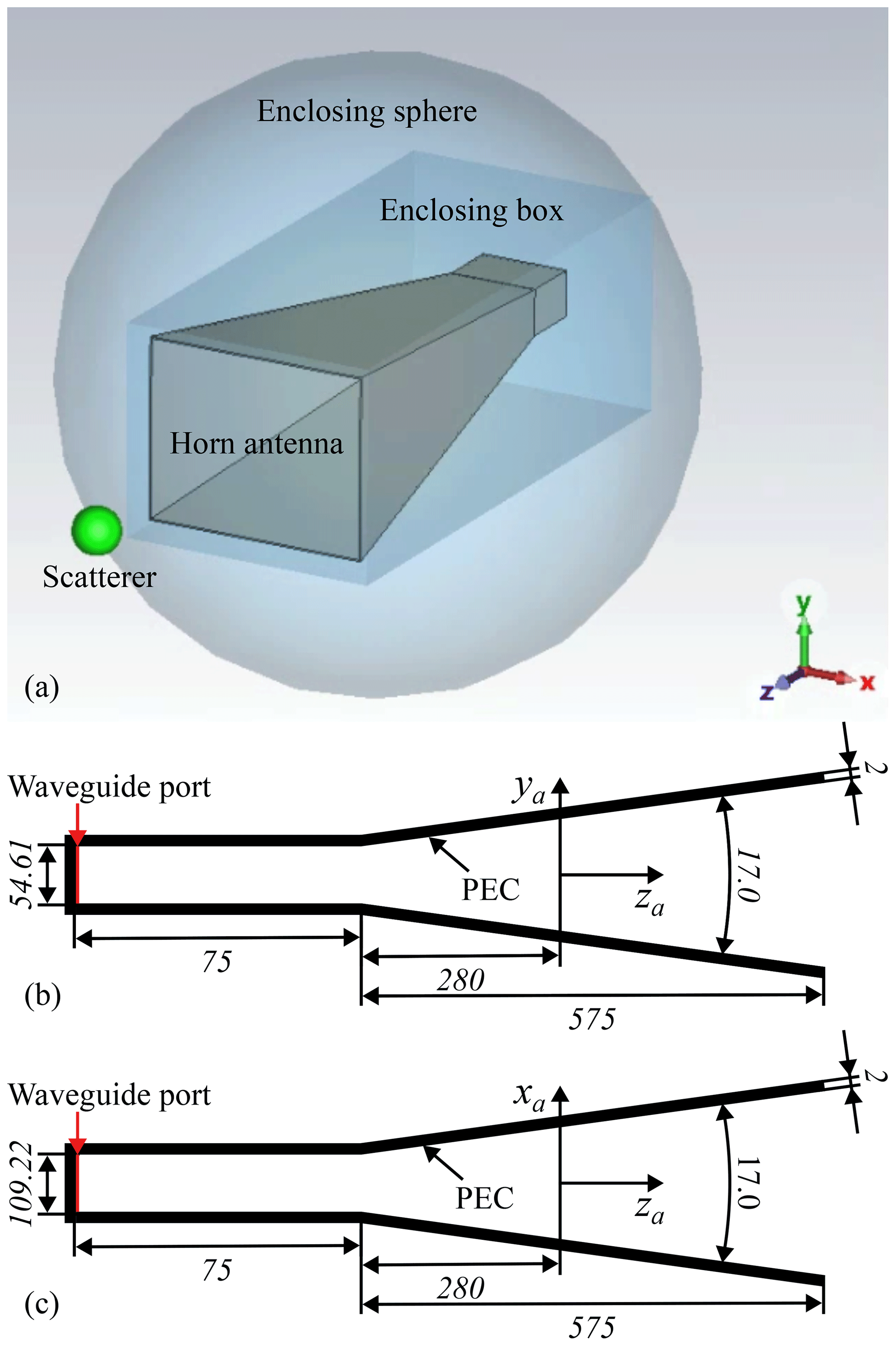
Figure 2 Horn antenna: (a) model in CST; (b) yz-cross section (not in scale); (c) xz-cross section (not in scale). The dimensions of the feeding rectangular waveguide are those of the WR430 standard. In (b) and (c), the taper angles are in degrees, while the other dimensions are in millimeters.

The parallelepiped has its sides orthogonal to either $i_{x^{\prime }}$, $i_{y^{\prime }}$, or $i_{z^{\prime }}$, its center in the antenna reference system is located at $(x_{\mathrm{a}}=\mathrm{0},y_{\mathrm{a}}=\mathrm{0},z_{\mathrm{a}}=-\mathrm{31})$ mm and the lengths of the x-,y-, and z-sides of the parallelepiped are 325.1 mm = 2.17λ, 270.5 mm = 1.80λ, and 692.0 mm = 4.62λ, respectively.

The matrix representations of the integral operators Eqs. (12), (13), (19), and (20) are evaluated numerically by applying the point matching method (Chew, 1995). The distance between the matching points is $\mathit{\lambda }/\mathrm{20}\approx \mathrm{7.5}$ mm and hence the total number of points over which the fields are exported is 18 322. For the value of the truncation limit N in Eq. (1), the following rule of thumb is applied (Hansen, 1988)

$$\begin{array}{}\text{(23)}& N=\lceil k_{\mathrm{s}}{R}_{\mathrm{s}}+\mathrm{10}\rceil =\mathrm{12}.\end{array}$$

For comparison with the classical approach based on the addition theorem (Stein, 1961) for VSMFs (Alian and Oraizi, 2018, 2019; Losenicky et al., 2021), the enclosing sphere with radius R_a=385 mm is also drawn in Fig. 2. Note that the enclosing sphere is more extensive than the enclosing box, thus limiting the minimum distance between the antenna's and scatterer's subdomains.

Two positions of the scatterer with respect to the reference system of the antenna are considered:

• P1: $O^{\prime }=(\mathrm{15},\mathrm{30},\mathrm{700})$ mm, r₀=700.8 mm;

• P2: $O^{\prime }=(\mathrm{0},\mathrm{0},\mathrm{375})$ mm, r₀=375.0 mm;

where r₀ is the distance between the origins of the two reference systems (Fig. 1). The electrical distances kr₀ are 29.4 and 15.7 for P1 and P2, respectively. Note that for P1, both the proposed method and the classical one based on the addition theorem for VSMFs can be applied. However, P2 can be analyzed only with the method proposed here, since in this case the sphere enclosing the antenna and the one enclosing the scatterer intersect.

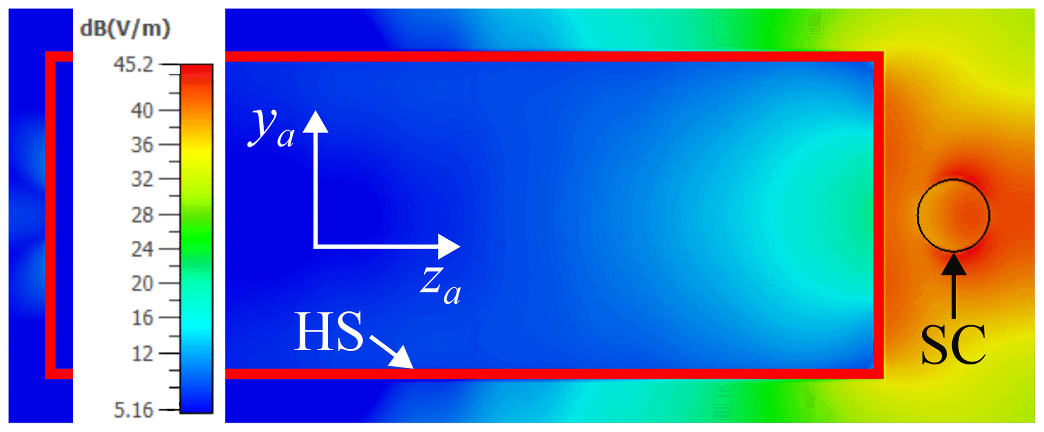
Figure 3 Equivalence principle in CST with scatterer in P2: maximum magnitude of the electric field on x_a=0 mm (Fig. 2b); HS stands for Huygens' surface while SC for scatterer.

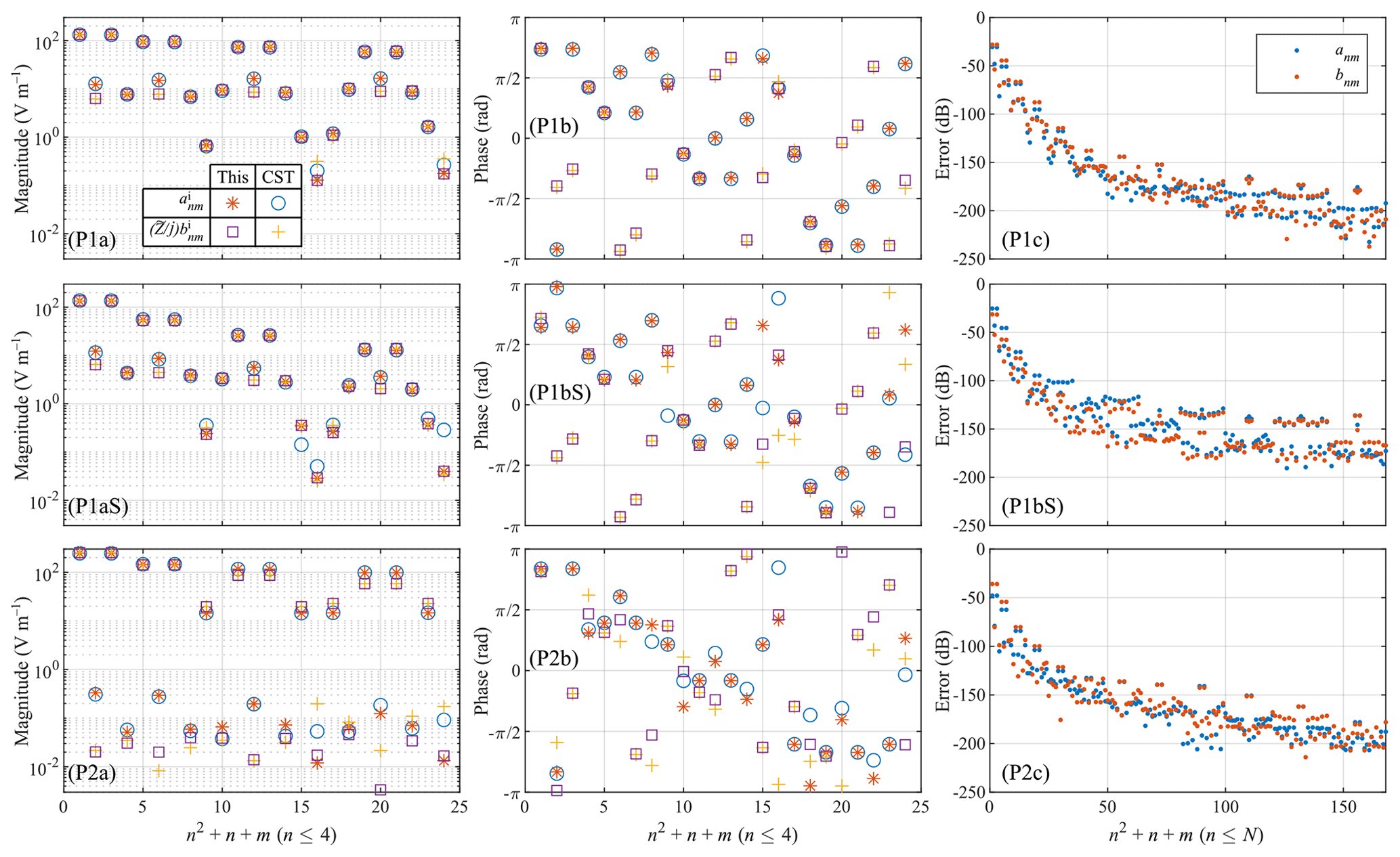
Figure 4 Coefficients of the multipole expansions: P1 or P2 indicates the position of the scatterer; a is for the magnitude, b the phase, and c the error Eq. (24); S, if present, indicates that the scatterer is considered. The legend of (P1a) is the same for all the graphs in the first two columns [without (with) scatterer $\stackrel{\mathrm{̃}}{Z}=Z$ ($\stackrel{\mathrm{̃}}{Z}=Z_{\mathrm{s}}$)]; the legend of (P1c) is the same for all the graphs in the third column.

A coupling between the scatterer and the antenna is expected, but this is not yet modeled by the proposed method. Therefore, to obtain CST results that are comparable with those of the proposed method, the CST reference solution is computed using the equivalence principle as follows:

• step 1: the subdomain of the antenna is solved and the equivalent currents on the bounding box are exported;

• step 2: the equivalent currents are loaded in CST as near-field sources and the antenna is replaced by the Huygens surface (Fig. 3).

Note that the field inside the Huygens surface in Fig. 3 does not vanish, which means that, as expected, there is an interaction between the antenna and the scatterer.

Once the proposed method is validated and no reference solution is further needed, it is sufficient to solve in CST only the subdomain of the antenna and to export the equivalent currents on the bounding box (step 1 of the aforementioned bullet list). The equivalent currents are then used as the input for the proposed method, which solves the scattering problem in the subdomain of the scatterer.

4.2 Comparisons

The multipole coefficients delivered by the proposed method and CST are now compared. Similarly to Hansen (2012), the relative error for this method (TM) and for the CST results is defined as

$$\begin{array}{}\text{(24)}& {\displaystyle }{\mathit{ϵ}}_{n,m}^c=\mathrm{20}\cdot {\log }_{\mathrm{10}}\left({\displaystyle \frac{\left|c_{n,m}^{\left(s\right)\mathrm{TM}}-c_{n,m}^{\left(s\right)\mathrm{CST}}\right|\cdot F_n}{{max}_{n,m}\left(\left|c_{n,m}^{\left(s\right)\mathrm{CST}}\right|\cdot F_n\right)}}\right)\text{(25)}& {\displaystyle }{F}_n={\displaystyle \frac{\mathrm{1}}{\sqrt{n}}}{\left({\displaystyle \frac{\mathrm{1}}{n}}\right)}^n\end{array}$$

where c is either a or b, and (s) is either (i) for the incident field or (in) for the field inside the scatterer. In Eq. (24), n and m range from 1 to N and from −n to n, respectively, as for the double summations in Eq. (1). The weighting factor F_n in Eq. (25) is necessary to account for the fact that the evaluation of the series Eq. (1) is convergent with n, but it is not for the series formed by the multipole amplitudes c_n,m. The reason for this can be found in the behaviour of the spherical Bessel function j_n(kr) which converge very fast for increasing n. Hence, we observe for the limit for n→∞ of the spherical Bessel function j_n(x):

$$\begin{array}{}\text{(26)}& j_n\left(x\right)\approx {\displaystyle \frac{\mathrm{1}}{\mathrm{2}\sqrt{xn}}}{\left({\displaystyle \frac{ex}{\mathrm{2}n}}\right)}^n\mathrm{for}n\to \mathrm{\infty }\end{array}$$

which thus makes Eq. (25) a suitable normalization factor in Eq. (24). On the other hand, F_n is closer to one for small values of n and it is exactly one for n=1. This means that the normalization factor F_n accordingly reduces the impact of the normalized multipole amplitudes for increasing values of n.

As an example, we first consider the multipole expansion in P1, with and without the scatterer, and second the multipole expansion in P2 without the scatterer.

For P1, the multipole coefficients of the incident electromagnetic field $a_{n,m}^{\mathrm{i}}$ and $(Z/j)b_{n,m}^{\mathrm{i}}$ are shown in Fig. 4 (first row) while those of the field inside the scatterer $a_{n,m}^{\mathrm{in}}$ and $(Z_{\mathrm{s}}/j)b_{n,m}^{\mathrm{in}}$ are shown in Fig. 4 (second row). The results agree well, except for slight discrepancies between the two methods that occur when the magnitude of the coefficients is less than 10⁰ V m⁻¹, i.e., become less relevant. The maximum value of the relative error Eq. (24) for $a_{n,m}^{\mathrm{i}}$ ($b_{n,m}^{\mathrm{i}}$) is −30.5 dB (−28.1 dB) and it is −25.2 dB (−31.3 dB) for $a_{n,m}^{\mathrm{in}}$ ($b_{n,m}^{\mathrm{in}}$).

For P1, electric fields are also qualitatively compared. The electric field of the impinging wave on a sphere with radius R_s is depicted in Fig. 5. We observe in both cases a similarity of the results from CST and the proposed method.

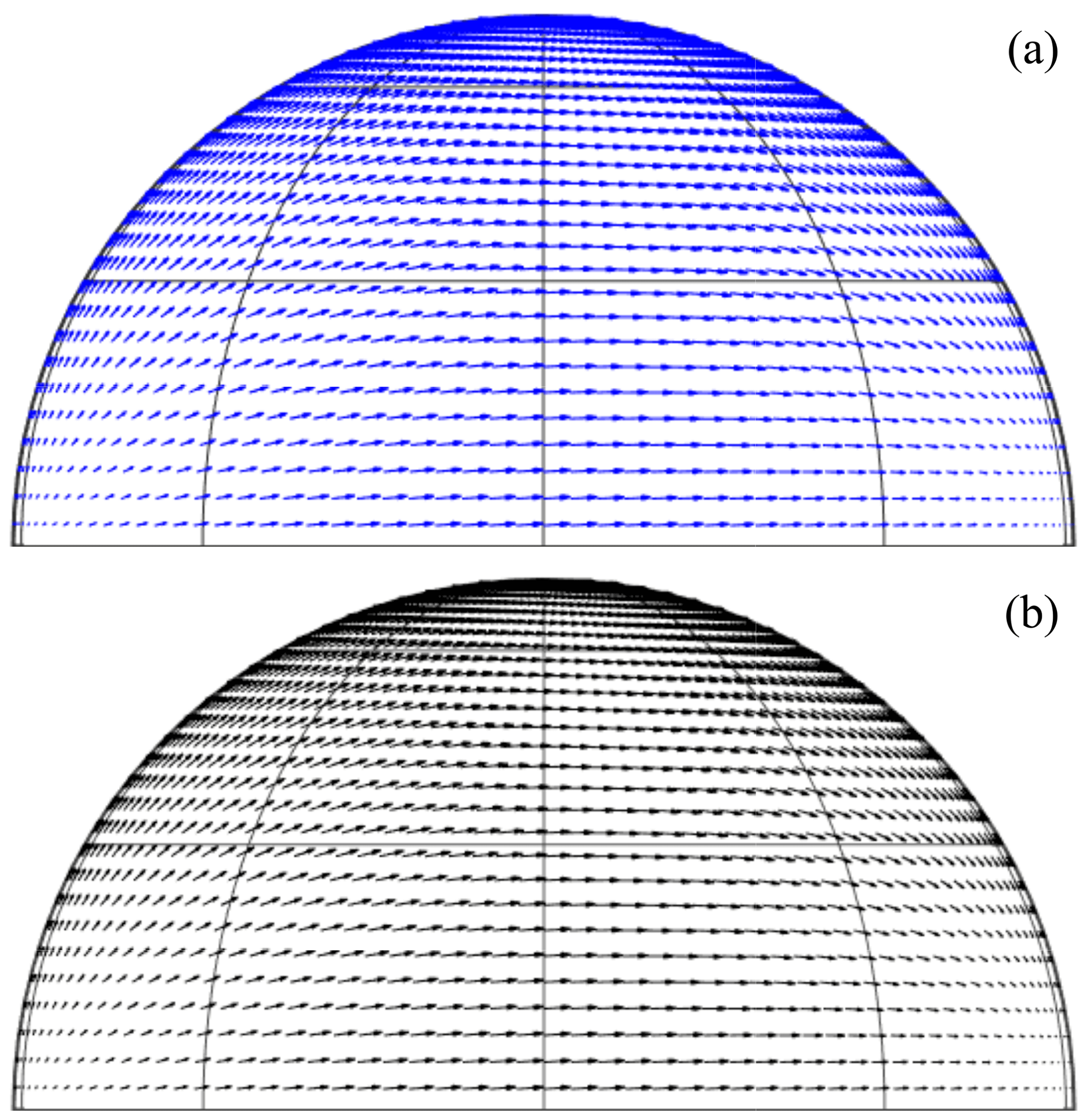
Figure 5 Projection of the incident electric field on the surface $r^{\prime }=R_{\mathrm{s}}$, $\mathrm{0}\le {\mathit{\phi }}^{\prime }\le \mathit{\pi }/\mathrm{2}$, $\mathrm{0}\le {\mathit{\theta }}^{\prime }\le \mathit{\pi }$ for the scatterer in P1: (a) proposed method; (b) CST.

For P2, the multipole coefficients of the incident field are shown in Fig. 4 (third row). For this case too, the results from the two methods agree well, apart for multipole amplitudes with a magnitude less than $\mathrm{2}\times {\mathrm{10}}^{-\mathrm{1}}$ V m⁻¹. The maximum value of the error Eq. (24) for $a_{n,m}^{\mathrm{i}}$ ($b_{n,m}^{\mathrm{i}}$) is −47.8 dB (−36.0 dB).

In Fig. 4 (third column), the error decreases fast for increasing multipole order for the term nⁿ in the denominator of the factor F_n. Due to this, the maximum value of the denominator in Eq. (25) is obtained for n=1 and $m=\pm \mathrm{1}$ in the examples analyzed. In addition, the relatively large values of the errors may derive from the limited accuracy of the CST reference solution. To support this, the maximum values of the errors are lower for the scatterer in P2, that is, for the scatterer closer to the antenna and hence a smaller solution domain in CST. The errors may decrease when solving the radiator with a dedicated solver.

5 Conclusions

We have introduced a method based on the dyadic Green's function and the equivalence principle to represent an electromagnetic field in a coordinate system different from the original one. The method works even when the classical approach based on VSMF translation formulas fails. This feature also allows one to reduce the distance between the antenna and the scatterer, particularly for elongated antennas. The proposed method has been compared to the numerical results purely obtained from the full-wave simulator CST, showing good agreement.

As the next step, the authors intend to solve the full scattering problem by including the electromagnetic interaction between different subdomains.