A hybrid algorithm to process millimeter wave images with prism-shaped aperture

To process images of a prism-shaped aperture in a radar imaging context, a hybrid algorithm is derived. This hybrid algorithm combines the benefits of backprojection and the Omega-K algorithm in terms of computational performance and flexibility. As a demonstration for an application of this algorithm, a 3D inspection system based on millimeter wave imaging is introduced. The system scans through the object, while it is passing on a conveyor belt. It comprises a curved antenna layout, which is able to synthesize the prism-shaped aperture. This aperture is shown to have superior resolution capabilities compared to a planar aperture. Some potential pitfalls when implementing the hybrid algorithm are assessed. Approximation formulae to estimate the achievable resolution are derived. The introduced algorithm is analyzed regarding its point spread function and compared to backprojection with the help of numerical simulations to demonstrate its potential.

1 Introduction

As soon as a company sells manufactured goods, it must ensure their quality or functionality (International Organization for Standardization, 2024). In addition to the optimization of production processes, quality control through automated testing processes is an important part of quality management as well. Over the last decades, the capabilities of machine learning frameworks for data analysis increased significantly. This enables producers to use industrial cameras for automated evaluation of quality. Cameras produce images with high resolution and are price-efficient compared to a manual inspection. But some production processes require a visual inspection through packaging or other opaque enclosing. To solve this problem, nowadays X-Ray inspection machines are used frequently. X-Ray produces high-resolution scans of the object's density distribution. The approach of using millimeter wave 3D radar imaging is newer in the industry and forms an alternative to other methods. Millimeter wave imaging visualizes contrast in the dielectric and conducting material properties of the object. Compared to X-Ray, its resolution is coarse due to the longer wavelength used. On the other hand, radar imaging devices do not emit ionizing radiation. The used electromagnetic waves in the power range of a few milliwatts are harmless to the human body and hence companies do not have to comply with potential radiation protection regulations.

This contribution presents a 3D radar imaging device targeted for applications in quality inspection and completeness checks. The system was first introduced as a conference contribution (Holder et al., 2024) along with preliminary experimental results. In this paper, a detailed derivation and analysis of the hybrid algorithm is given. An approximation for the theoretical resolution limit is derived and tested using numerical simulations. The device is capable of processing data in real-time and directly transferring images to a potential evaluation unit via a generic camera interface. Thus, the device is designed to be readily used in an industrial application. The device is mounted on top of a conveyor belt and images an object under test (OUT), while it is passing underneath. Several submodules, equipped with radar measurement MMICs, illuminate the OUT from different perspectives, while it is moving. Therefore, it is possible to make use of inverse synthetic aperture techniques.

Many different geometries for the aperture have been investigated in the past. These include circular apertures (Soumekh, 1999), segments of a cylinder or a sphere (Fortuny-Guasch and Lopez-Sanchez, 2001), as well as complete cylinders (Vaupel, 2016). The effect of the illumination angle for planar imaging is investigated by Ahmed et al. (2010). Various acquisition schemes for cylindrical radar imaging were investigated in a security environment. Most solutions include a MIMO approach along with movement of the antennas to reduce the hardware effort (Gao et al., 2018; Berland et al., 2022; Li et al., 2021a).

In this paper, a signal processing algorithm is developed to process the acquired raw data into a 3D image. A detailed description of the developed algorithm and a comparison with the backprojection algorithm along with numerical simulations is given. The remainder of this paper is organized as follows. Section 2 delivers a detailed description of the used radar imaging device. In the beginning of Sect. 3, backprojection and the Omega-K algorithm are briefly described, followed by the introduction and analysis of a novel hybrid processing algorithm. The theoretical resolution limits of the introduced imaging device are derived. Section 4 compares the introduced algorithm with backprojection and analyzes the achieved resolution limits in a simulated environment. At last, Sect. 5 draws a conclusion and gives an outlook into future work.

2 Device description

The introduced radar imaging system is a modification of the RadarImager (Balluff GmbH, 2025) from Balluff GmbH, a commercially available quality inspection machine based on millimeter waves. The extension overcomes the limitations of a planar aperture by using frontend measurement submodules in a curved arrangement. This is depicted in Fig. 1. Deploying a curved aperture around the OUT has several benefits. First, the effect of shadowing through specular reflections is reduced due to the higher variety of possible wave paths. Inclined surfaces have a higher probability of getting illuminated properly, such that a receiving antenna is able to capture its reflection. Second, the resolution of the image is improved, as derived and demonstrated later in this paper.

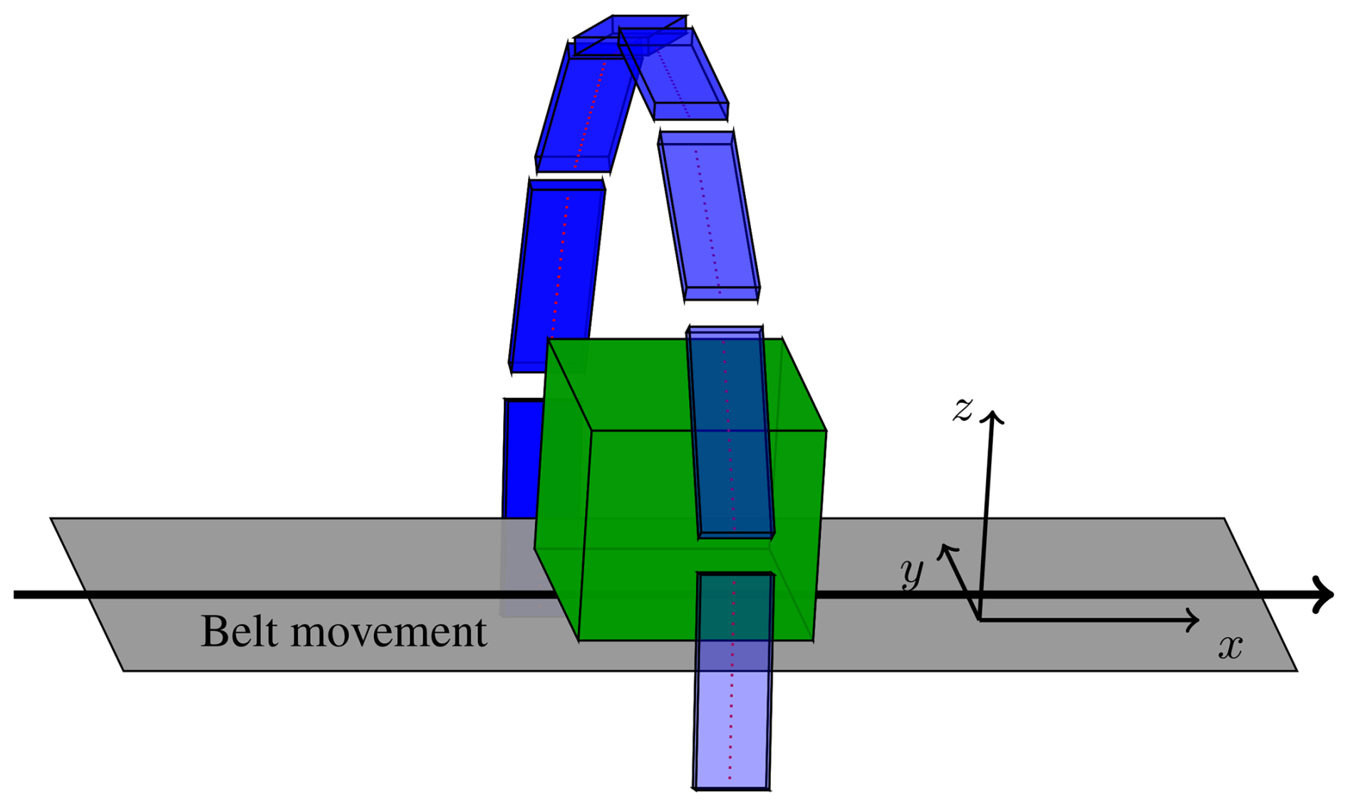
Figure 1 Sideview pictogram of the radar imaging device. The submodules (blue) comprise a line of virtual antennas (red dots). The green box represents an OUT.

The system comprises an active radar aperture as well as powerful embedded computing hardware, which computes radar images from the captured signals directly on the device. The 3D radar images are immediately outputted in an easily interpretable image format through a standardized camera interface. The radar aperture is composed of eight submodules. Position and orientation of these submodules can be adjusted to realize different aperture shapes. Each submodule is a printed circuit board with 16 commercially available radar MMICs installed. Each radar MMIC has four closely spaced antenna channels included inside the chip package. Additional digital controllers for a coordinated control flow are present on the submodules. A picture of the system showing its submodules is depicted in Fig. 2.

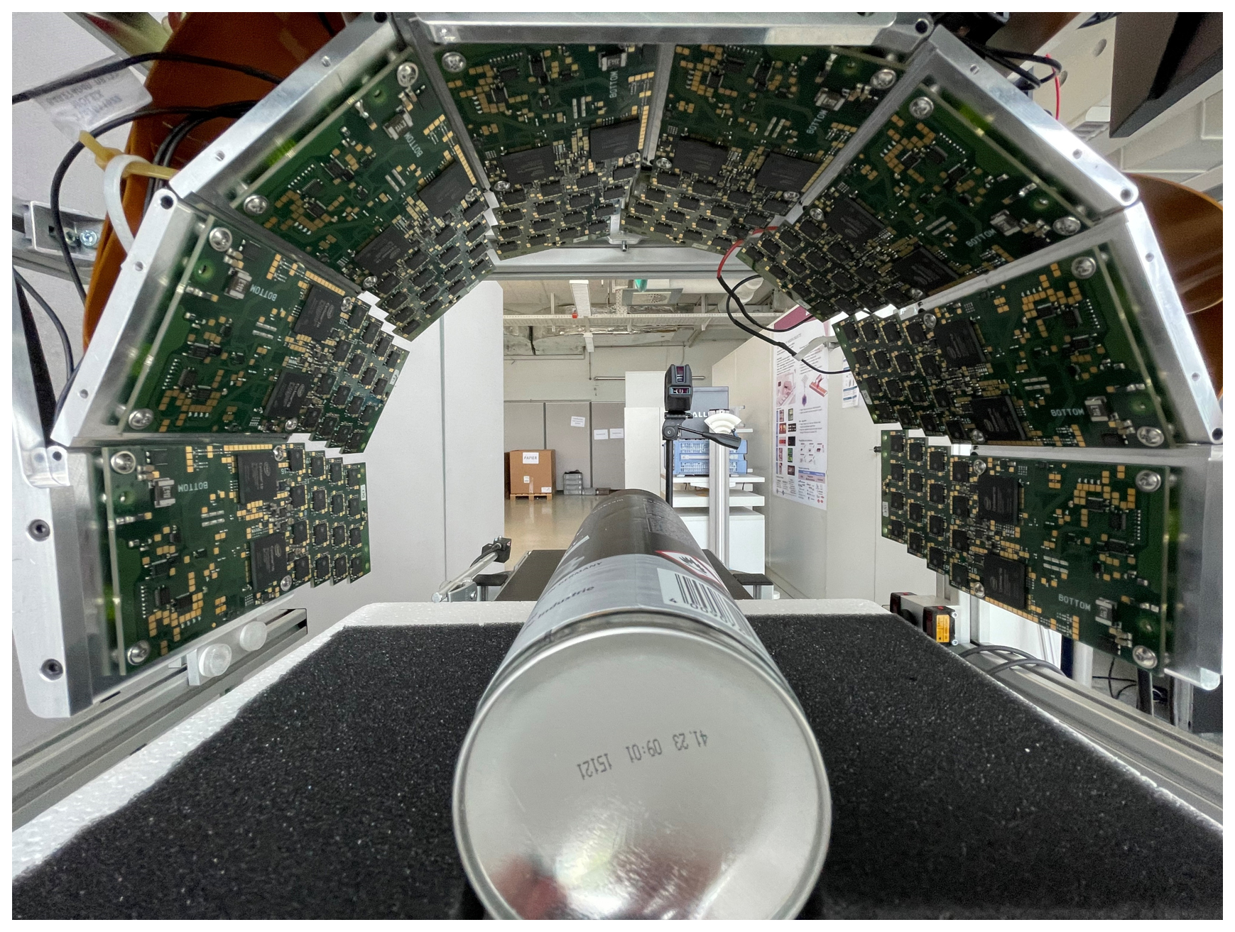
Figure 2 Frontview picture of the device showing its frontend submodules. A spraycan represents an exemplary OUT.

The radar MMICs operate in the V-Band from 57.1 to 63.9 GHz. An on-chip transmitter antenna emits frequency modulated continuous-wave (FMCW) chirps. Each of the four receiver antennas captures the signals scattered at the OUT and, after downconversion, the so called beat signal is digitized. Applying the concept of virtual antennas, the transmitter and the four receiver antennas inside the MMIC yield a four channel monostatic aperture. Note that the MMICs itself are not coupled and operate individually. In order to avoid interference between the numerous radar MMICs, their operation is synchronized and temporally arranged using time division multiplexing (TDM).

Eight submodules, each containing 16 MMICs, which in turn each comprise 4 virtual antennas, result in a total of N_A=512 antenna elements. While the OUT is passing on the conveyor belt, a central control flow unit generates trigger pulses. Each pulse leads to a measurement event. The conveyor belt speed and the trigger pulse rate is synchronized, such that the belt travel between two events is Δ_x=1 mm. Therefore, the Nyquist criterion of ${\mathrm{\Delta }}_x\le {\mathit{\lambda }}_{\min }/\mathrm{4}$ is fulfilled for the used frequency range. At an event, each of the N_A virtual channels performs a radar measurement of the OUT. After receiving an event, the FMCW chirps are sequentially transmitted through TDM. The net measurement time of one event is in the microseconds range. Thus, although the chirps are not performed at the exact same time, the OUT movement during an event can be neglected.

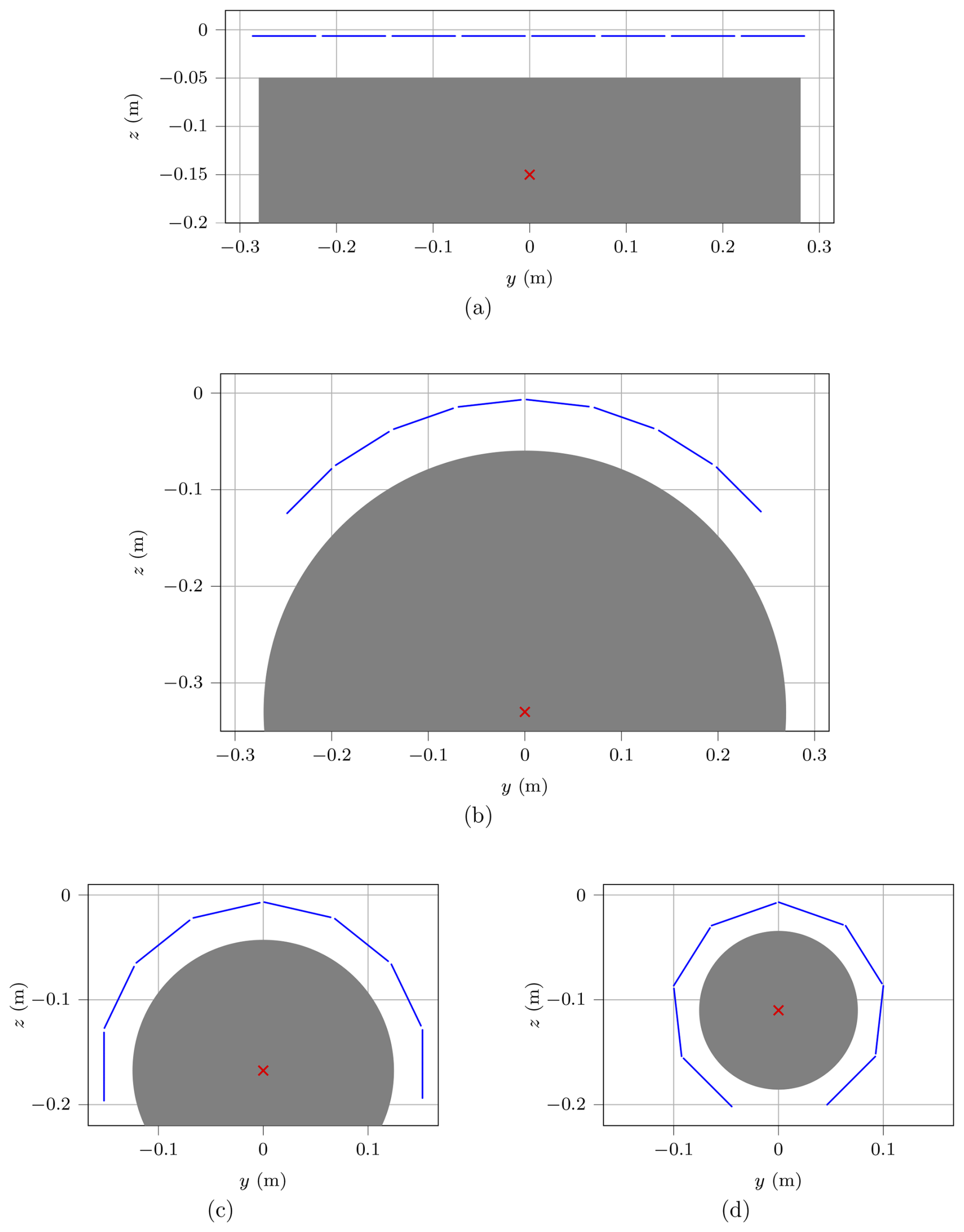
Figure 3 Antenna positions projected on yz-plane for the four geometric configurations. The virtual antenna aperture is shown in blue. Gray area shows the maximum extent of the OUT (projected on yz-plane). The red cross depicts the simulated scatterer location in Sect. 4. (a) Flat configuration, (b) 90° configuration, (c) 180° configuration, (d) 270° configuration.

Four geometrical configurations of the submodules, from flat up to a three-quarter turn are investigated. They are shown in Fig. 3.

For simplicity of the following derivations, it makes sense to introduce a moving coordinate system. The new cartesian coordinate system is chosen to have its x-axis parallel to the movement of the conveyor belt and its origin moves with the exact same velocity. From a perspective of this new coordinates, the OUT is now static, while the antennas are passing parallel to the negative x-axis. The y and z components of the moving coordinate system are chosen to coincide with the origin shown in Fig. 3. As visible in Fig. 2 the radar MMICs are staggered in four rows along the conveyor direction (parallel to the x-axis). Let the physical position of ith antenna be given by the position vector ${\mathit{p}}_i=(x_i,y_i,z_i{)}^{⊺}$.

The x-component of antenna i is now dependent on the event index n, if expressed in the moving coordinate system and given by $x_i^{\prime }=x_i-n\cdot {\mathrm{\Delta }}_x$. As a preprocessing step, the effect of different antenna positions x_i on the aperture is eliminated with an index shift. A simplified antenna layout of one submodule is illustrated in Fig. 4. This hypothetical antenna array depicted consists of 8 antennas and an antenna offset along the x direction of 2⋅Δ_x. Note that the real antenna distribution of the 64 antennas per submodule is slightly more complex, but follows a similar scheme. The event-based data from each antenna is now organized to create a uniform sample array. This is achieved by sorting and shifting the individual data streams. The concept is visualized in Fig. 5. Note that for the first and last few event-indices n, only some of the antennas contribute to the raw data set. In the following, the number of net shifted samples along x_p will be denoted as N_x≤N_Events.

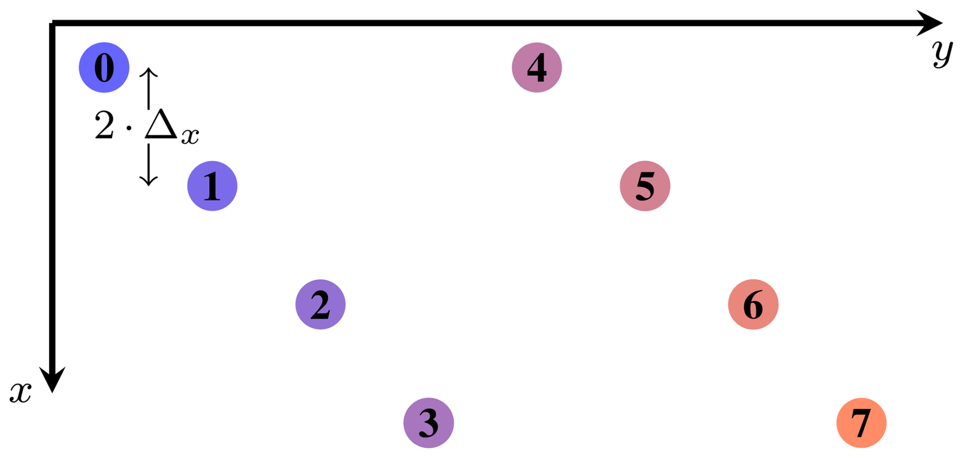
Figure 4 Hypothetical antenna layout of one submodule (xy-plane) with antenna indices 0 to 7.

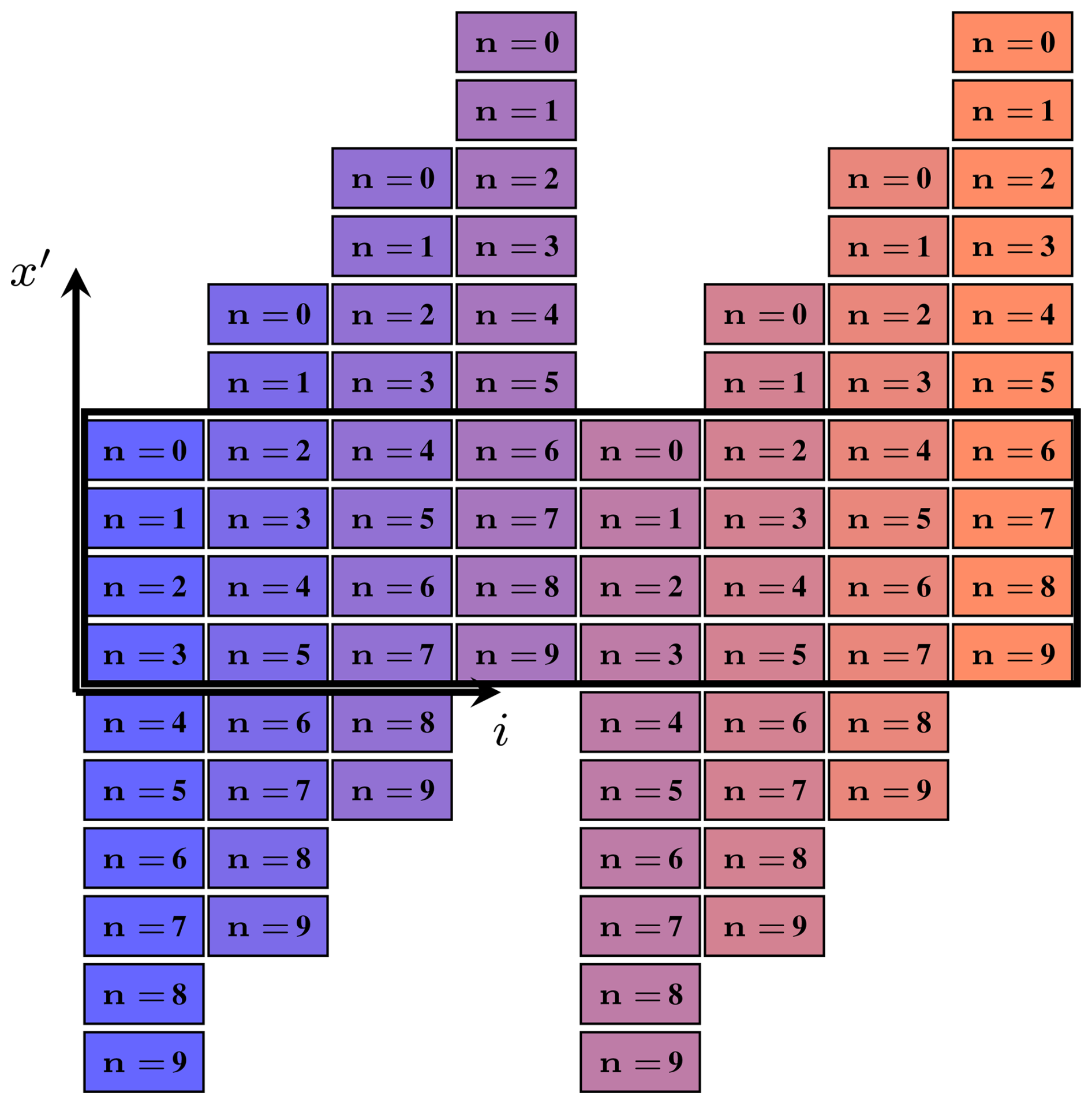
Figure 5 Visualization of the concept of event reordering by index shift. Samples from different antenna indices i are shaded into different colors. The black box surrounds the net used data for further processing.

The three-dimensional raw data set is now defined as $S(n,i,j)$ for further processing. $n\in [\mathrm{0},N_x-\mathrm{1}]$ denotes the event index, $i\in [\mathrm{0},N_{\mathrm{A}}-\mathrm{1}]$ gives the used antenna and $j\in [\mathrm{0},N_{\mathrm{f}}-\mathrm{1}]$ denotes the frequency index of the complex-valued sample.

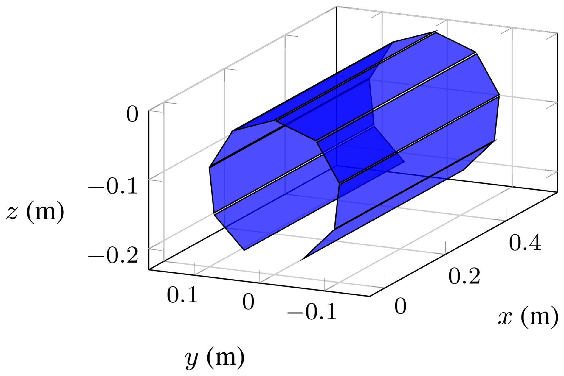
After the reordering step, the assembled synthetic aperture of S forms the shape of an open prism, depending on the chosen geometric configuration. The generated aperture shape for the 270° configuration is shown in Fig. 6 as an example.

Figure 6 Synthetic aperture of the 270° configuration.

3 Imaging algorithm

This section gives an overview over the millimeter Wave imaging algorithms backprojection and Omega-K. Thereafter, the novel hybrid algorithm is introduced. In general, millimeter wave imaging has the goal to characterize an object by means of a reflectivity function g(r), which is a complex-valued function over space $\mathit{r}=(x,y,z{)}^{⊺}$. The functions support is restricted by the OUTs size. In this derivation, scaling components are omitted for the sake of simplicity. The aim is now to approximate g(r) with millimeter wave scattering measurements as precisely as possible. Usually, the underlying signal model for reconstruction makes use of the Born approximation. With this approximation, the total field at each scattering point is equivalent to the incident field. In effect, each scatterer contributes individually to the received signal and does not interact with other parts of the OUT. Pan and Kak (1983) derived the approximation for the case of a plane wave illuminating the OUT. Additionally, it is assumed, that the g(r) does not alter over frequency. A transmitting antenna illuminates the OUT with electromagnetic waves over varying frequency f. For a FMCW chirp, this frequency changes constantly over time in a given bandwidth. The derived wavenumber $k=\mathrm{2}\mathit{\pi }f/c_{\mathrm{0}}$ therefore varies as well from k_min to k_max, where c₀ denotes the speed of light.

The received antenna signal of a monostatic radar measurement is proportional to the amplitude of the backscattered electric field at location p, which is given by

$$\begin{array}{}\text{(1)}& S(\mathit{p},k)=\iiint g\left(\mathit{r}\right)\cdot w(\mathit{p},\mathit{r})\cdot e^{-j\cdot \mathrm{2}k\cdot |\mathit{r}-\mathit{p}|}\mathrm{d}\mathit{r}.\end{array}$$

w(p,r) describes an arbitrary weighting function used to model antenna gain, free space loss or other effects on the signal amplitude. The phase term of the signal in Eq. (1), only depends on the relative distance between scattering point and antenna. Therefore, it is possible to define g(r) in the moving coordinate system introduced in Sect. 2. In the following, the generic signal S(p,k) will be replaced with the introduced specific raw data format $S(n,i,j)$.

3.1 Backprojection algorithm

The backprojection algorithm is based on a matched filter calculation for the individual response signatures of a point scatterer. The response signature is dependent on the location r of the scatterer. The imaging result $\widehat{g}$ for one pixel at r is given by

$$\begin{array}{}\text{(2)}& \begin{array}{rl}\widehat{g}\left(\mathit{r}\right)=& \sum _{n=\mathrm{0}}^{N_x-\mathrm{1}}\sum _{i=\mathrm{0}}^{N_{\mathrm{A}}-\mathrm{1}}\underset{k_{\min }}{\overset{k_{\max }}{\int }}S(n,i,k)\cdot w\left({\mathit{p}}_i\right(n),\mathit{r})\\ & \cdot e^{+j\cdot \mathrm{2}k\cdot |\mathit{r}-{\mathit{p}}_i(n\left)\right|}\mathrm{d}k.\end{array}\end{array}$$

The inner integral over the wavenumber k reduces to a sum, since the radar responses are sampled through the FMCW chirp. Note that this triple sum has to be computed for each point r of the image. To optimize the computation time of the backprojection algorithm, an inverse FFT is used to correlate the samples of one Chirp (Li et al., 2021b). By using a Fourier transform for each chirp, a signal $S(n,i,t)$ is obtained. The dimension t can be rescaled into the range domain with $R=t/\mathrm{2}{c}_{\mathrm{0}}$. The backprojection algorithm can now be reformulated to

$$\begin{array}{}\text{(3)}& \widehat{g}\left(\mathit{r}\right)=\sum _{n=\mathrm{0}}^{N_x-\mathrm{1}}\sum _{i=\mathrm{0}}^{N_{\mathrm{A}}-\mathrm{1}}S\left(n,i,{\displaystyle \frac{|\mathit{r}-{\mathit{p}}_i(n\left)\right|}{\mathrm{2}{c}_{\mathrm{0}}}}\right)\cdot e^{+j\cdot \mathrm{2}k\cdot |\mathit{r}-{\mathit{p}}_i(n\left)\right|}.\end{array}$$

The mathematical equivalence of Eqs. (2) and (3) is shown by Gorham and Moore (2010). When implementing the backprojection algorithm, $\frac{|\mathit{r}-{\mathit{p}}_i(n\left)\right|}{\mathrm{2}{c}_{\mathrm{0}}}$ can be an arbitrary real number and therefore $S\left(n,i,\frac{|\mathit{r}-{\mathit{p}}_i(n\left)\right|}{\mathrm{2}{c}_{\mathrm{0}}}\right)$ needs to be interpolated accordingly. For this contribution, linear interpolation is used as a trade-of between computational effort and accuracy. Zero-padding is used along with the inverse FFT to increase the number of sampling support points along R.

3.2 Omega-K algorithm

The Omega-K algorithm, also called range migration algorithm, uses a decomposition of the recorded data into plane waves. For this, a three-dimensional set of samples $S(x,y,k)$ is required. The samples along x and y must be equidistantly arranged in a plane. To decompose into plane waves, a 2D Fourier transform over x and y is performed. The spatial spectral domain of a signal is called k-space. Applying the 2D Fourier transform yields

$$\begin{array}{}\text{(4)}& S(k_x,k_y,k)={\mathcal{F}}_{x,y}\left(S(x,y,k)\right).\end{array}$$

With the scalar wavenumber k, the dispersion equation

$$\begin{array}{}\text{(5)}& k_z=\sqrt{\mathrm{4}{k}^{\mathrm{2}}-\mathrm{4}{k}_x^{\mathrm{2}}-\mathrm{4}{k}_y^{\mathrm{2}}}\end{array}$$

can be applied. The transformed signal can therefore be expressed as non-uniform samples of $S(k_x,k_y,k_z)$. The support of $S(k_x,k_y,k_z)$ forms the shape of a spherical shell, as shown by Sheen et al. (2001). By using a 1D interpolation, the so-called Stolt interpolation, along k_z, the samples can be arranged into an arbitrarily defined regular grid from k_z,min to k_z,max. The grid should be chosen large enough, to cover all sample points. Afterwards, a 3D inverse Fourier transform can be applied to obtain

$$\begin{array}{}\text{(6)}& I^{\prime }(x,y,z)={\mathcal{F}}_{k_x,k_y,k_z}^{-\mathrm{1}}\left(S(k_x,k_y,k_z)\right).\end{array}$$

The Fourier transform is applied through a 3D IFFT in the discrete domain. Since the IFFT is applied on a shifted support ($k_{z,\min }\ne \mathrm{0}$), a phase correction step

$$\begin{array}{}\text{(7)}& I(x,y,z)=I^{\prime }(x,y,z)\cdot e^{j\cdot \mathrm{2}{k}_{z,\min }\cdot z}\end{array}$$

is necessary. In its basic form, the Omega-K algorithm is restricted to produce images, where the geometric pixel grid of $I(x,y,z)$ matches the sample grid of $S(x,y,k)$. If scattering occurs outside the sampling area, described by the box from ($x_{\min },x_{\max },y_{\min },y_{\max }$), the 3D IFFT wraps the signal contributions into the image. Scattering contributions are located to the wrong position and thus will distort the image region of interest. By the introduction of zero-padding, this restriction can be overcome. A new signal $S_{\mathrm{pad}}(x,y,k)$ is defined by

$$\begin{array}{}\text{(8)}& \begin{array}{rl}& S_{\mathrm{pad}}(x,y,k)=\\ & \left\{\begin{array}{ll}S(x,y,k),& \mathrm{if}{x}_{\min }\le x\le x_{\max }\wedge y_{\min }\le y\le y_{\max }\\ \mathrm{0},& \mathrm{else}\end{array}\right.\end{array}\end{array}$$

After padding, $S_{\mathrm{pad}}(x,y,k)$ is used as the argument in Eq. (4). Although filled with zeros, the added spatial regions in the processed image $I(x,y,z)$ are not necessarily empty. Scattering points can still be represented with a reduced resolution. Let the padding factor F_p be defined as the ratio between original and padded size of the dataset in xy-plane.

Although the Omega-K algorithm has more processing steps and includes more complex scaling and interpolation, Omega-K is computationally efficient, because both discrete Fourier transforms can be implemented with the FFT algorithm.

3.3 Hybrid algorithm to process prism shaped apertures

The backprojection algorithm can be applied flexibly to almost any geometric configuration and produces accurate results. On the other hand, its computational complexity makes the backprojection algorithm infeasible for many time critical applications. On the other hand, the Omega-K algorithm is only capable of handling planar apertures. To find a feasible solution for the introduced aperture shape in Sect. 2, a hybrid algorithm is developed.

Restructuring the summing components from Eq. (3)

$$\begin{array}{}\text{(9)}& \begin{array}{rl}\widehat{g}\left(\mathit{r}\right)=& \sum _{i_M=\mathrm{0}}^{\mathrm{7}}(\sum _{n=\mathrm{0}}^{N_x-\mathrm{1}}\sum _{i=\mathrm{0}}^{\mathrm{63}}S\left(n,i^{\prime },{\displaystyle \frac{|\mathit{r}-{\mathit{p}}_{i^{\prime }}(n\left)\right|}{\mathrm{2}{c}_{\mathrm{0}}}}\right)\\ & \cdot e^{+j\cdot \mathrm{2}k\cdot |\mathit{r}-{\mathit{p}}_{i^{\prime }}(n\left)\right|}).\end{array}\end{array}$$

where i_M denotes the submodule index and $i^{\prime }=\mathrm{64}\cdot i_M+i$ with $\mathrm{0}\le i\le \mathrm{63}$ gives an interesting insight. The backprojection algorithm computes a subimage for each submodule and finally adds them together, when structured like in Eq. (9). The inner sums can be replaced by a subimage $g_{i_M}\left(\mathit{r}\right)$ computed with the data from submodule i_M only. Moving from backprojection to the novel hybrid algorithm, the inner part of Eq. (9) is altered. Since the eight subimages originate from a planar aperture, the Omega-K algorithm can be applied individually. Let $I_{i_M}(x,y,z)$ be defined as the resulting image, when using only submodule i_M as input data. At first, each subimage $I_{i_M}$ is defined in its own coordinate system with position vectors ${\mathit{r}}_{i_M}=(x,y_{i_M},z_{i_M}{)}^{⊺}$, where the $x{y}_{i_M}$-plane coincides with the individual circuit board surface. Before performing an addition, the subimages must be projected into a common coordinate system. The projected subimage is given by

$$\begin{array}{}\text{(10)}& I_{p,i_M}(x,y,z)=I_{i_M}\left(\mathcal{P}(x,y_{i_M},z_{i_M}{)}^{⊺}\right).\end{array}$$

The projection operator 𝒫 is defined on any position vector by

$$\begin{array}{}\text{(11)}& \begin{array}{rl}\mathcal{P}\left(\begin{array}{c}x\\ y_{i_M}\\ z_{i_M}\end{array}\right)=& \left(\begin{array}{ccc}\mathrm{1}& \mathrm{0}& \mathrm{0}\\ \mathrm{0}& \cos \left({\mathit{\varphi }}_{i_M}\right)& -\sin \left({\mathit{\varphi }}_{i_M}\right)\\ \mathrm{0}& \sin \left({\mathit{\varphi }}_{i_M}\right)& \cos \left({\mathit{\varphi }}_{i_M}\right)\end{array}\right)\\ & \cdot \left({\mathit{r}}_{i_M}-{\mathit{p}}_{\mathrm{0},i_M}\right).\end{array}\end{array}$$

The submodules rotation angle ${\mathit{\varphi }}_{i_M}$ is given by

$$\begin{array}{}\text{(12)}& {\mathit{\varphi }}_{i_M}={\displaystyle \frac{\left(i_M-\mathrm{7}/\mathrm{2}\right)}{\mathrm{7}}}\cdot {\mathit{\theta }}_{\mathrm{c}}\end{array}$$

and the origin base vector ${\mathit{p}}_{\mathrm{0},i_M}$ of each vector, which is given the position of the leftmost aperture point for this subimage. θ_c denotes the maximum viewing angle each for the given geometric configuration. After projection, the subimages don't fit into a regular pixelgrid. Interpolation in the yz-plane is necessary to match the individual $I_{p,i_M}(x,y,z)$ on a common pixel grid. In this contribution, bilinear interpolation is used. The hybrid algorithm is then described by

$$\begin{array}{}\text{(13)}& \widehat{g}\left(\mathit{r}\right)=\sum _{i_M=\mathrm{0}}^{\mathrm{7}}{I}_{p,i_M}(x,y,z).\end{array}$$

When applying the phase correction of Eq. (7), the signal gets a strong phase variation over z. This can lead to challenges in the interpolation step. Therefore, the authors chose to apply the projection before the phase correction step. Equation (13) can then be reformulated to

$$\begin{array}{}\text{(14)}& \widehat{g}\left(\mathit{r}\right)=\sum _{i_M=\mathrm{0}}^{\mathrm{7}}{I}_{i_M}^{\prime }\left(\mathcal{P}\left(x_{i_M},y_{i_M},z_{i_M}\right)\right)\cdot e^{j\cdot \mathrm{2}{k}_{z,\min }\cdot z}.\end{array}$$

Another aspect to keep in mind regarding the interpolation step, is the phase drift over z. When performing the Omega-K algorithm, the main signal contribution in k-space typically lies in the upper part of the obtained shell (refer to Fig. 7). Choosing a low k_z,min could potentially cover high lateral resolution (high k_x and k_y) signal components and lead to higher resolution images. On the other hand, choosing a low k_z,min shifts the largest signal contributions further away from k_z,min. This leads to faster phase fluctuations in $I^{\prime }(x,y,z)$ making them harder to interpolate when adding the subimages together.

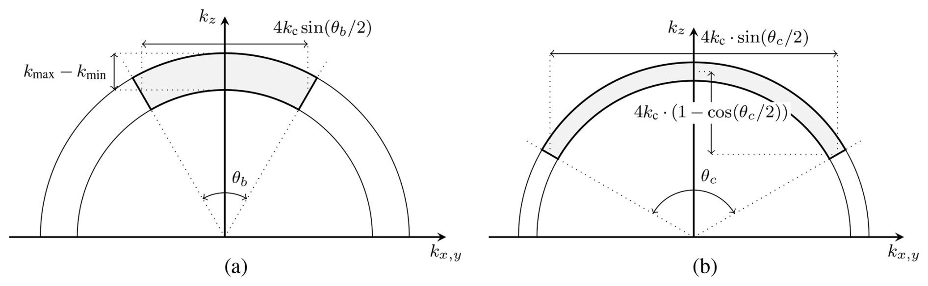
Figure 7 Methods to approximate the k-space support sizes. (a) Typical approach, (b) proposed approach.

When using the hybrid algorithm, it is crucial to use zeropadding as described in Sect. 3.2 to adapt to the maximum OUT expansion around the focal point (Holder et al., 2024). The focal point of the configuration is the point in the yz-plane where the normal vector of each submodule is pointing to. For the flat configuration, no such focal point can be defined.

3.4 Resolution

The critical distance δ, where two objects can still be separated in an image is defined as the resolution. To give an approximation for theoretical resolution the extent of a scene in k-space is investigated. Therefore, the spherical support of the object in k-space is approximated by a rectangular shape. In the case, where the antenna pattern limits the resolution in flat configurations, the resolution in cross-range (x and y dimensions) and range (z-dimension) is typically given by

$$\begin{array}{}\text{(15)}& {\mathit{\delta }}_{x,y}={\displaystyle \frac{{\mathit{\lambda }}_{\mathrm{c}}}{\mathrm{4}\cdot \sin ({\mathit{\theta }}_{\mathrm{b}}/\mathrm{2})}}\end{array}$$

and

$$\begin{array}{}\text{(16)}& {\mathit{\delta }}_z={\displaystyle \frac{c_{\mathrm{0}}}{\mathrm{2}B}}.\end{array}$$

respectively (Sheen et al., 2001), where λ_c denotes the center wavelength, θ_b the opening angle of the antenna and B the bandwidth of the system. This is given by the inverse widths of the slab thickness in k_x,y or k_z.

Another way to find out the resolution is to derive the point spread function (PSF) and determine the width of its main-lobe. The PSF is defined as the response of an imaging system for a point-like source. For a full circular imaging geometry, Berizzi and Corsini (1999) calculated a resolution of ${\mathit{\delta }}_{x,y}\approxeq \mathrm{0.19}{\mathit{\lambda }}_{\mathrm{c}}$. Note, that this is less than the achievable optimum of ${\mathit{\lambda }}_{\mathrm{c}}/\mathrm{4}$ with Eq. (15). The shape of the PSF is dependent on the position of the scatterer and therefore, the resolution can vary in different image regions as well.

In order to find the resolution for the presented four geometric configurations, θ_b is now replaced by the viewing angle extent θ_c at the focus point of the aperture. By assuming that B is small compared to the center frequency f_c, the width of the k-space coverage can be calculated with the help of θ_c. This results in a range resolution

$$\begin{array}{}\text{(17)}& {\mathit{\delta }}_z={\displaystyle \frac{{\mathit{\lambda }}_{\mathrm{c}}}{\mathrm{2}\cdot \left(\mathrm{1}-\cos ({\mathit{\theta }}_{\mathrm{c}}/\mathrm{2})\right)}}\end{array}$$

and a cross-range resolution perpendicular to the conveyor belt

$$\begin{array}{}\text{(18)}& {\mathit{\delta }}_y=\left\{\begin{array}{ll}\frac{{\mathit{\lambda }}_{\mathrm{c}}}{\mathrm{4}\sin ({\mathit{\theta }}_{\mathrm{c}}/\mathrm{2})},& {\mathit{\theta }}_{\mathrm{c}}\le \mathit{\pi }\\ \frac{{\mathit{\lambda }}_{\mathrm{c}}}{\mathrm{4}},& {\mathit{\theta }}_{\mathrm{c}}>\mathit{\pi }\end{array}\right.\end{array}$$

Using ${\mathit{\theta }}_{\mathrm{c}}=\mathit{\{}\mathit{\pi }/\mathrm{2},\mathit{\pi },\mathrm{3}\mathit{\pi }/\mathrm{2}\mathit{\}}$ for the Config 90°, Config 180° and Config 270° respectively, the individual resolution results can be obtained using Eqs. (15) to (18). To calculate the resolution in x direction, the simulated antenna 3dB-beamwidth of 40° is inserted. The resolution δ_x is the same for all configurations since the effective aperture along the conveyor belt stays the same.

4 Numerical Simulations

This section investigates the proposed hybrid algorithm by using simulated data as input. The simulation uses Eq. (1) to compute $S(n,i,j)$ for a single point-like scatterer. To simulate an antenna pattern, the angle between the antenna's normal vector and p_s−p_i is computed. p_s denotes the position of the simulated scatterer. This acts as input for the weighting function w(⋅). A radial symmetric antenna pattern with an opening angle of θ_b=40° is assumed. The antenna pattern is a simple constant gain main-lobe tapered off in the interval $\mathrm{15}\mathit{°}<\left|\mathit{\theta }\right|<\mathrm{25}$°. The boundary region is modeled with a raised cosine function and no side-lobes are simulated for the antenna pattern. The free-space loss was not considered for simulation. This simplification is sufficient for simulations of a single, center-positioned scatterer.

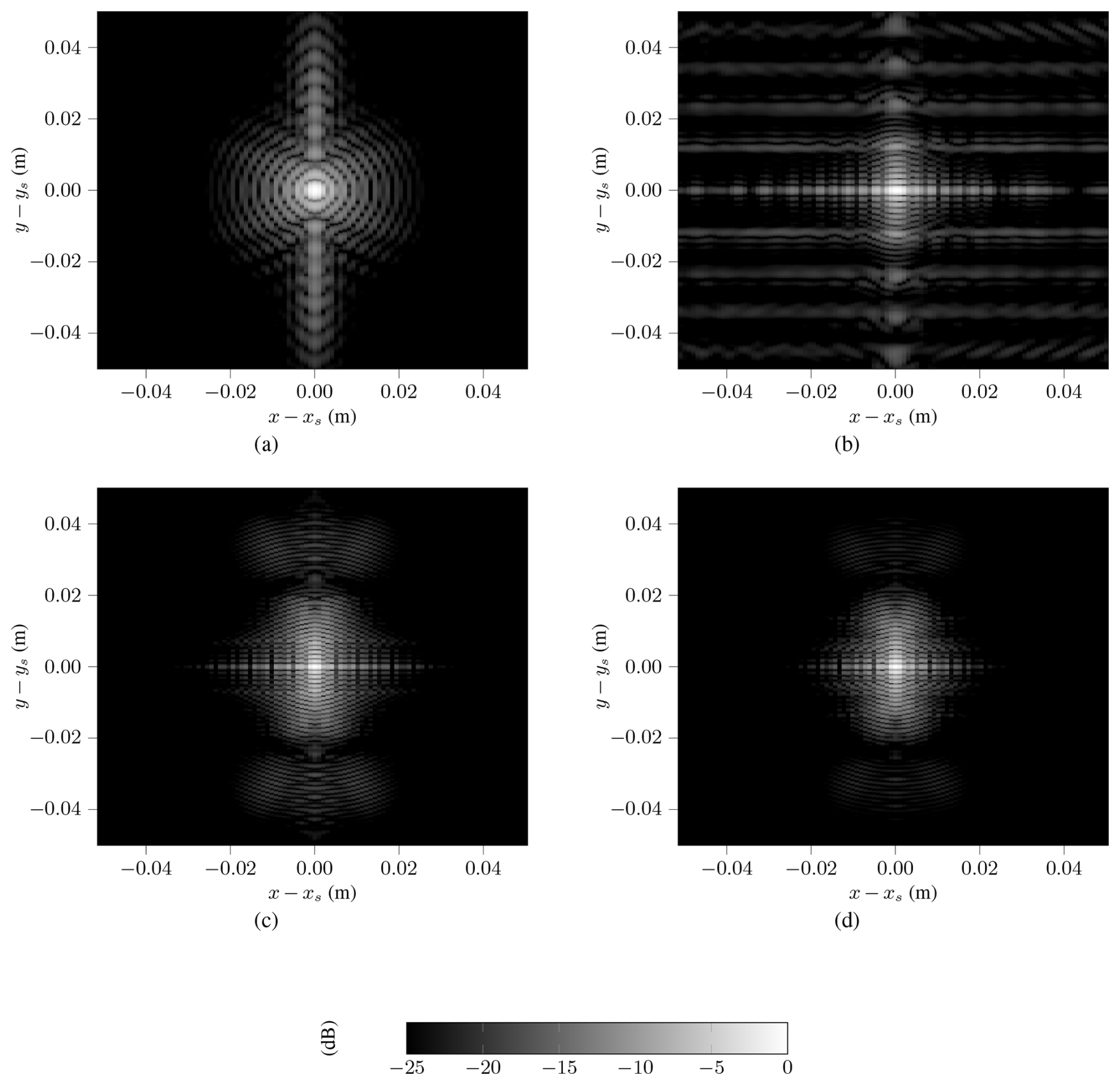
Figure 8 PSF for a scatterer simulated at the configurations focal point (dB) for (a) Config flat, (b) Config 90°, (c) Config 180° and (d) Config 270°.

First the PSF of the hybrid algorithm is investigated. The simulated scatterer was placed at the focal point for each of the curved configurations. So the scatterer locations are ${\mathit{p}}_{\mathrm{s}}=(\mathrm{0.1}\mathrm{m},\mathrm{0}\mathrm{m},-\mathrm{0.33}\mathrm{m})$, ${\mathit{p}}_{\mathrm{s}}=(\mathrm{0.1}\mathrm{m},\mathrm{0}\mathrm{m},-\mathrm{0.1675}\mathrm{m})$ and ${\mathit{p}}_{\mathrm{s}}=(\mathrm{0.1}\mathrm{m},\mathrm{0}\mathrm{m},-\mathrm{0.11}\mathrm{m})$ for the Configurations 90, 180 and 270°, respectively. For the flat configuration, ${\mathit{p}}_{\mathrm{s}}=(\mathrm{0.1}\mathrm{m},\mathrm{0}\mathrm{m},-\mathrm{0.15}\mathrm{m})$ was chosen as a moderate distance. The simulated scatterer locations are shown as red crosses in Fig. 3. The hybrid algorithm uses F_p=2 as a padding factor and applies window functions before of its each Fourier transforms. Applying a 3D window function in k-space effects the resolution as well as the sidelobe levels in the processed subimages. Figure 8 shows the PSF for each of the configurations as a cut in xy-plane. The structure of the PSF has different shapes, depending on the chosen configuration. It can be observed, that the main lobes width decreases with increasing curvature. For the 90° configuration, horizontal artifacts can be seen. These sidelobes originate from an artifact of the simulation boundary. The scatterer has the highest distance and its full radar response was not completely covered in the simulated data. To investigate the achieved resolutions in more detail and to compare them with the theoretical results from Sect. 3.4, cuts along each dimension are shown in Fig. 9. The results obtained with the backprojection algorithm are shown as well for comparison.

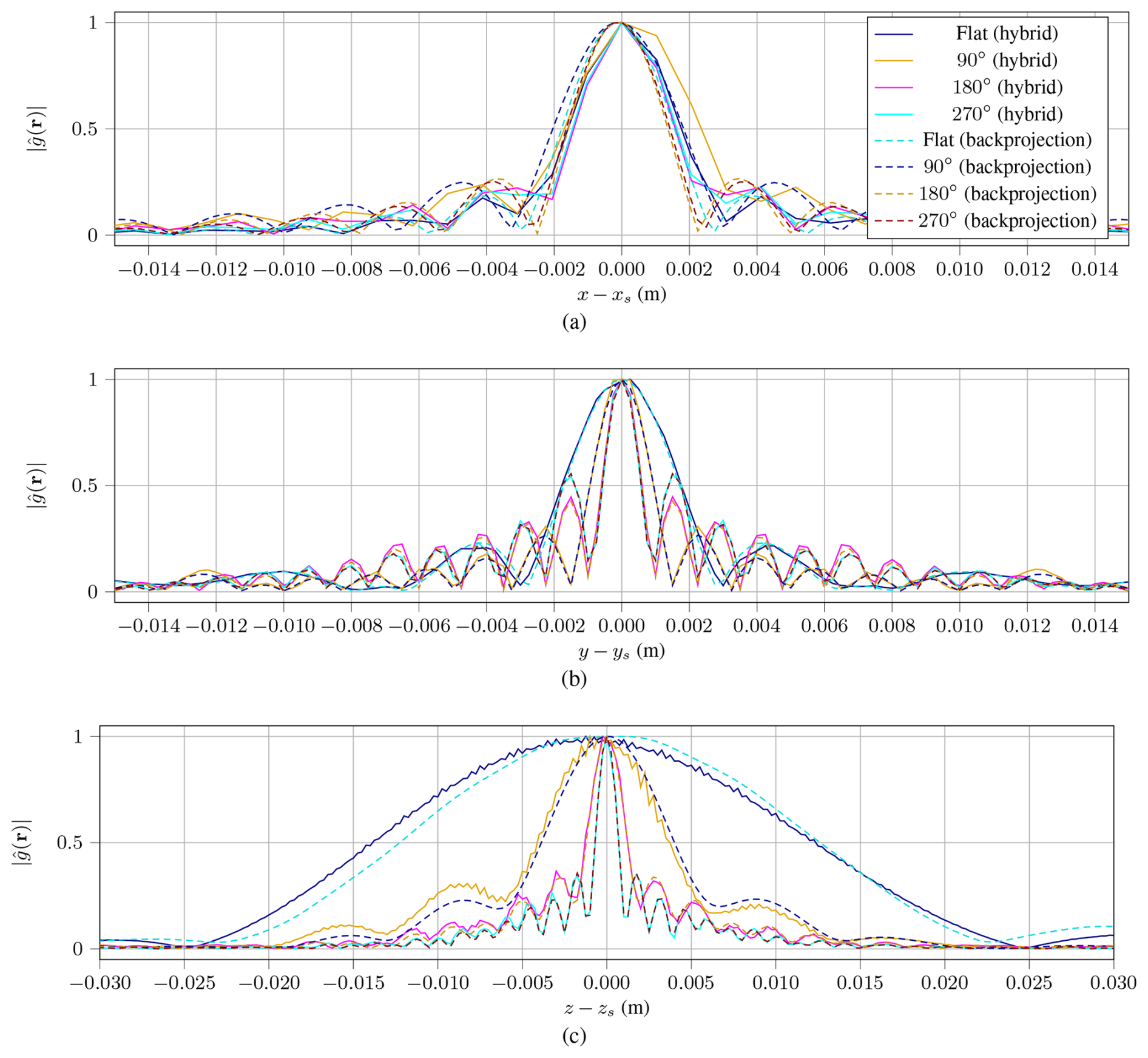
Figure 9 Comparison of PSF for all Configurations (a) along x-axis, (b) along y-axis and (c) along z-axis.

For the 90, 180 and 270° configs, the resulting PSFs are very similar between the backprojection and the hybrid algorithm.

Along the z-axis, the PSFs procuded by the hybrid algorithm exhibit a noisy component, particularly in the flat and 90° configurations. The curves are less smooth compared to those obtained through backprojection processing. This noise arises from the rapid fluctuations in phase of the subimages along the z-axis, which makes interpolation more challenging.

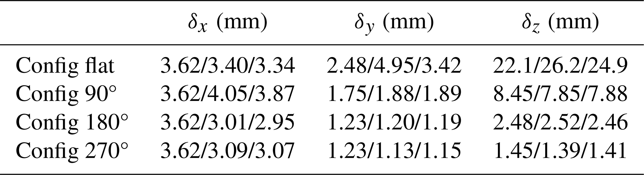
From the results shown in Fig. 9, the achieved resolutions in each dimension are determined. Therefore, the 3 dB-width of the mainlobe is measured and collected in Table 1. They are compared to the theoretical results calculated for simulated parameters using Eqs. (15) to (18). Regardless of the chosen algorithm, it is observable, that the theoretical resolution δ_x is not achieved for the 90° configuration. As mentioned earlier, the aperture is limited to the measurement length instead of the antenna pattern, which makes the approximation invalid for this case. For the other three configurations, the achieved resolution along x is even better than the calculated result, although the bandwidth along k_x is limited by the opening angle of the antenna. This behavior requires further investigation. The derived formulas for δ_y and δ_z seem to get more accurate for larger θ_c. This makes sense, because the deviation of a bandwidth B becomes more and more neglectable. In two cases, the simulated resolution is slightly better than the calculated theoretical resolution limit. This probably originates from the approximation B=0. Additionally it underlines, that Eqs. (17) and (18) are just an approximation to the mathematical exact resolution limit for the given geometry. As mentioned before, implementation details like zero-padding, windowing and other filtering operations can influence the resolution as well.

Table 1 Resolution results compared (theoretical/hybrid/backprojection).

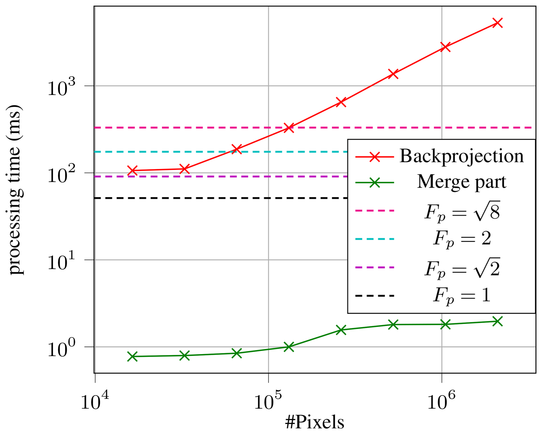
To evaluate the computational performance of the introduced hybrid algorithm, a comparison with backprojection regarding execution time was executed. Both algorithms were executed using parallel computing on a Nvidia GeForce RTX3080 Ti Laptop GPU. The input data of a simulated single scattering point is used. A datatset $S(n,i,j)$ with N_x=256 and the system configuration in Config 90° is simulated. Both algorithms compute the same image region of $\mathrm{10}\times \mathrm{10}\times \mathrm{10}$ cm with varying granularity of pixels. The number of total pixels is swept from 16384 up to roughly 2 million pixel points. Figure 10 depicts the processing time of backprojection and the hybrid algorithm. For the backprojection algorithm, the processing time scales linearly with the number of image pixels. For the hybrid algorithm, the processing time stays nearly constant. The only processing step scaling with the number of output pixels is the final merging step. As seen in Fig. 10, the projection and addition part scales roughly in a linear manner. But the absolute execution time only varies from ≈ 1.1 to 2.4 ms. The main contribution for to processing time forms the computation of the eight subimages via Omega-K. It can be observed, that the complexity scales linearly with the padding factor F_p. Overall, it can be seen, that making use of the introduced hybrid algorithm leads to a significant performance benefit, especially for larger OUTs.

Figure 10 Execution times for different problem sizes.

5 Conclusions

To optimize the resolution and angular extent of illumination, an industrial millimeter wave inspection machine was modified. The device was transformed into a system with a curved aperture, which uses the movement of a conveyor belt to generate a 3D aperture with the shape of an open prism. To adapt to the shape of the object to be inspected, the aperture can be physically adjusted into four geometric configurations. A novel processing algorithm, which acts as a hybrid between the backprojection and the Omega-K algorithm, was derived. A method to approximate the theoretical resolution of each imaging geometry was given and compared to simulated resolution results. The hybrid algorithm was shown to yield similar imaging results to the backprojection algorithm, while significantly lowering the computational complexity. The obtained resolution by an approximation formula and simulation were compared. The accuracy of the approximations derived is especially good for higher curvatures. For some cases, the simulated resolution does not match with the expected resolution very well. It is especially remarkable, that the resolution along the height axes of the prism is affected by the apertures overall curvature. Several cases show a better resolution in simulation than given by the approximation formula. This can be explained by signal processing details like windowing functions, but needs more detailed investigation for the cases with larger deviation. As expected, the achievable resolution improves significantly using a prism shaped aperture compared to a flat one. With the introduction of a fast hybrid algorithm, the system is able to process the data in real-time on an industrial GPU. The other potential benefit of a curved system, the improved illumination properties, will be investigated in more detail in a future paper. The problem of system alignment, already described in the authors previous contribution, will be tackled as well in the near future.