Long-term changes and trends of mesosphere/lower thermosphere gravity waves over Collm, Germany

Time series of mesosphere/lower thermosphere half-hourly winds over Collm (51.3° N, 13.0° E) have been obtained from 1984–2007 by low frequency (LF) spaced receiver measurements and from 2004 to date by very high frequency (VHF) meteor radar Doppler wind observations in the height range 82–97 km. These observations are analysed with respect to gravity wave (GW) climatology and trends. From half-hourly differences of zonal and meridional winds, GW variance proxies have been calculated that describe amplitude variations in the period range 1–3 h. After applying corrections to account for instrumental differences, the GW climatology and time series have been obtained. The mean GW activity in the upper mesosphere shows maximum amplitudes in summer, while in the lower thermosphere GWs maximize in winter. At altitudes around 90 km, positive/negative long-term trends are visible in winter/summer, consistent with increasing/decreasing mesospheric winds. In the lower thermosphere, however, long-term amplitude trends are generally positive. We notice qualitative correspondence of these trends with those derived from satellite observations of potential energy despite of different wavelength ranges seen by radar and satellite. Quasi-decadal and interannual variations of GW amplitudes and mean winds are also visible, showing a possible influence of the 11-year solar cycle or lower atmosphere circulation patterns.

1 Introduction

Gravity waves (GWs) couple the lower atmosphere and the mesosphere/lower thermosphere (MLT) region at 80–100 km and also the thermosphere/ionosphere. They are filtered by the middle atmosphere wind jets, so that their distribution and variability at MLT heights reflect the dynamical conditions below. On the other hand, GWs deposit momentum to the mean flow of the upper atmosphere, and therefore they are important for maintaining the circulation of the MLT and thermosphere. Thus, observations of GW and their variability and trends are necessary to obtain a comprehensive picture of MLT and thermospheric wind and temperature drivers, and to interpret long-term variations of the upper atmosphere dynamics in connection with lower atmosphere climate variability and trends.

Long-term observations of upper-atmosphere GWs are sparse. Oliver et al. (2013) indicated that GW activity at ionospheric altitudes could be increasing since the 1970s. Hydroxyl airglow observations in Zvenigorod (56° N, 37° E) 2000–2024 also showed a positive trend at about 87 km (Perminov et al., 2024). Limited observations from radar and from space showed that GW trends in the middle atmosphere are regional and unstable. Hoffmann et al. (2011) reported positive GW trends over Northern Germany from 1990–2011 in the height range 80 to 88 km. On the other hand, Jacobi (2014a) reported negative trends above 83 km in summer and a weak indication of positive trends below. These observations referred to the time interval 1984–2007. Over North America, Gardner and She (2022) reported a decrease of GW amplitudes from the 1990s to the 2000s based on Ft. Collins (41° N, 105° W) and Starfire Optical Range (35° N, 106.5° W) lidar observations. They attributed this to a decrease of precipitation events since the year 2000. Since over Europe the negative trend is not seen in each month of the year, regional effects may play a role here. Earlier, Gavrilov et al. (2002) has shown that interannual GW variations from Canada, Europe, and Japan, all at Northern Hemisphere midlatitudes, showed considerable differences, which the authors attributed to different GW sources or GW propagation conditions. From 14 years of satellite observations (2002–2015), Liu et al. (2017) reported insignificant trends during most months in the midlatitude MLT, but negative trends in July. Since the time intervals considered by these investigations differ, the contradicting results may indicate unstable trends. However, the considered GW period ranges and observational filters of the different methods may as well influence the results.

To summarize, it is unclear, whether or not GWs at MLT heights exhibit long-term trends. To enlarge the available database of GW proxies, we here present long-term analyses of wind variances from 1984 to June 2024, based on wind observations made at Collm (51.3° N, 13.0° E). The time series consists of data obtained with two different methods that will be described in the following section, as well as the method of calculation of the GW proxies, and the combination of the data based on different measurements.

2 Observations

At Collm, MLT winds had been measured from December 1959 to 2008 by the low frequency (LF) spaced receiver (D1) method (e.g., Sprenger and Schminder, 1967) using the sky wave of different commercial radio transmitters, including Zehlendorf near Berlin on 177 kHz. The lower ionospheric reflection point of the 177 kHz sky wave registered at Collm was located at 52.11° N, 13.21° E. Half-hourly horizontal winds have been analysed using the similar fade method at three receivers at Collm with 300 m distance (e.g., Schminder and Kürschner, 1994). The applied method made use of the fact that corresponding maxima or minima of similar fadings of the sky wave were registered at the different receivers with a time delay with respect to each other, which is proportional to the drift velocity of electron density fluctuation patterns at the LF reflection height near 90 km.

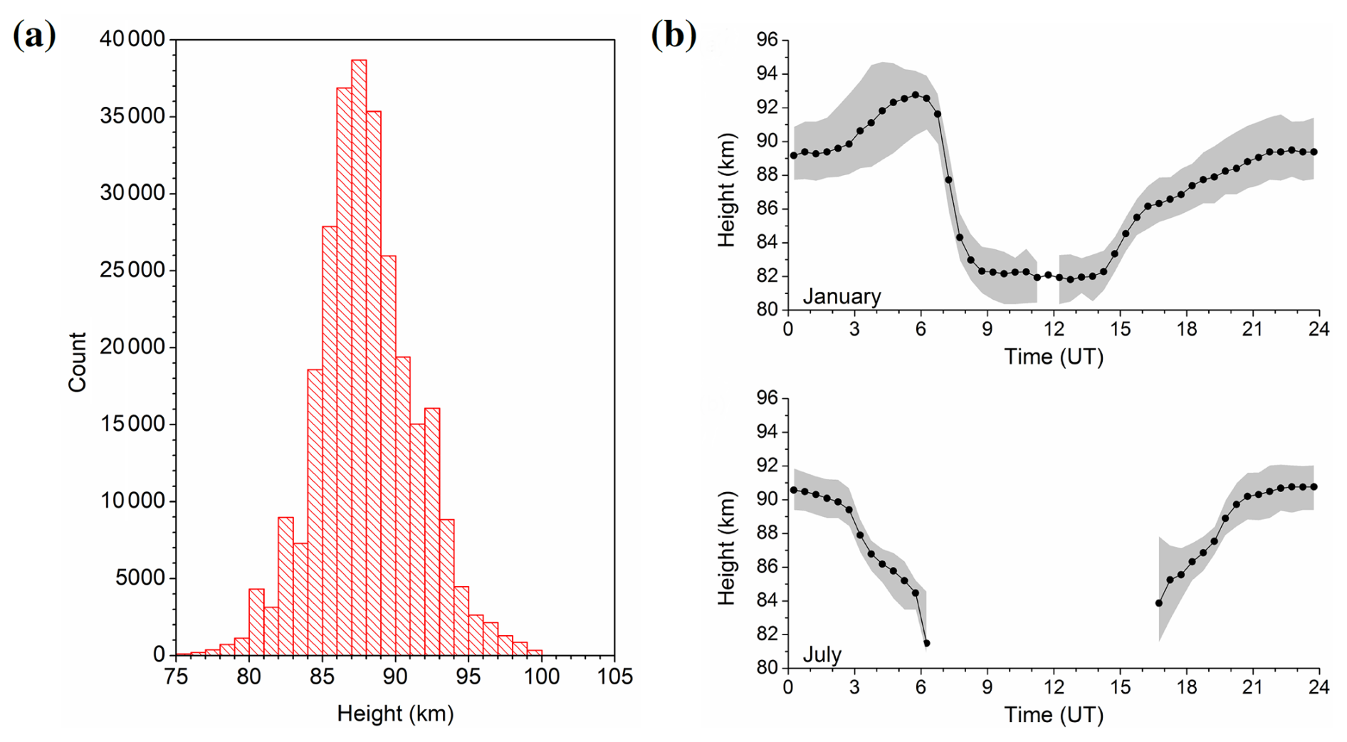
Figure 1 Corrected LF mean reflection heights. (a) Histogram based on data 1984–August 2007 (b) diurnal cycle for January (top) and July (bottom) 1983–2007. Greyshading indicates upper and lower quartiles, if enough data for calculating these are available.

LF reflection heights have been observed since 1983 until 2007 by phase comparisons of the ground wave and the sky wave in a modulation frequency band near 1.8 kHz (Kürschner et al., 1987). Due to group retardation the estimated virtual heights are too large, and have been corrected here using an empirical reduction factor based on phase comparisons of the solar semidiurnal tide derived from LF and very high frequency (VHF) meteor radar (MR) observations (Jacobi, 2011). Distributions of the corrected heights are shown in Fig. 1. Note that the reflection heights are changing during the day, and at lower heights around 82 km observations were only possible in winter during daylight hours. During summer observations became sparse and data gaps appear due to LF radio wave absorption in the ionospheric D region in the mesosphere.

Since 2004 to date, VHF MR observations on 36.2 MHz have been performed at Collm using the Doppler shifted radio waves reflected from underdense meteor trails. An upgrade of the radar has been made in 2015/2016, including antenna configuration and peak power increase. Details of the radar configuration can be found, e.g., in Stober et al. (2021). The radar delivers winds in the approximate height range of 75–105 km. The height information is provided by an interferometer. The data are binned here in six not overlapping height gates centred at 82, 85, 88, 91, 94, and 98 km with 3 km width, with an exception for the upper gate with 5 km width. Individual winds calculated from the meteors are collected to form half-hourly mean values using a least squares fit of the horizontal wind components to the raw data under the assumption that vertical winds are small (Hocking et al., 2001). The nominal heights not necessarily correspond to the mean heights within the gates, because the meteor rates maximize closely below 90 km and decrease above and below that height (e.g., Jacobi, 2014b). Therefore, above the meteor maximum the real mean heights are lower than the nominal heights. However, a substantial difference is only visible for 98 km nominal altitude, so that the real mean height of the uppermost gate is closer to 97 km than 98 km (Jacobi, 2012).

To estimate deviations $u^{\prime },v^{\prime }$ from the LF half-hourly means, a simple method is applied by using the halved differences of two subsequent half-hourly mean winds and analysing the variances ${u^{\prime }}^{\mathrm{2}},{v^{\prime }}^{\mathrm{2}}$ according to Gavrilov et al. (2001, 2002). Note that variances are not included in the further analysis, if the height changes by more than Δh=2 km from one half-hourly mean to another. The limit Δh was chosen as a compromise between reducing the effect of wind shear, and the need for a sufficiently large number of data. The LF data are sorted into six different height gates of 6 km width centred at 82, 85, 88, 91, 94, and 97 km, i.e. at the same height as the MR mean heights, but with larger bin width. Monthly mean variances are calculated, and seasonal means are taken as averages over three monthly means. For the MR observations, half-hourly wind values attributed to the same heights as for the LF values are used, and variances are calculated as for the LF observations.

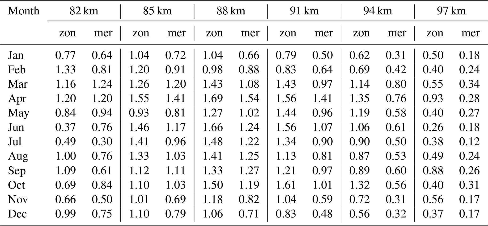
LF and MR winds and thus resulting variances have been obtained by quite different methods. Therefore, we expect that variances obtained by the two methods differ. In particular, meridional LF winds show a bias towards smaller amplitudes (Jacobi et al., 2009). Here we did not perform a mean wind correction such as, e.g., in Jacobi et al. (2015), but directly corrected the variances based on their comparison during the period of overlapping measurements from August 2004 to August 2007. We made a comparison of LF $/$ MR variances for each month, and for each height gate separately. This was necessary because in particular in summer there were data gaps during daylight hours, and only few observations were made at lower heights (see Fig. 1). Furthermore, the diurnal distribution of heights was uneven due to the diurnal lower ionospheric E region change, so that possible diurnal cycles of GW amplitude would lead to different biases at different heights. Furthermore, as has been shown, e.g., by Jacobi et al. (2009), the LF winds at the upper height gates show an increasing negative bias. Finally, spaced receiver observations tend to overestimate zonal winds with respect to the meridional ones, so that the corrections have been made for each horizontal wind component separately. The LF $/$ MR bias correction factors are provided in Table A1 in Appendix A. Examples for uncorrected and corrected LF variances at 88 km together with MR values are shown in Fig. 2. Uncorrected zonal LF variances are somewhat larger than MR ones at this height gate, while the meridional components are similar for both methods at that height. From the resulting time series we note a clear seasonal cycle, as well as some interannual and quasi-decadal variability.

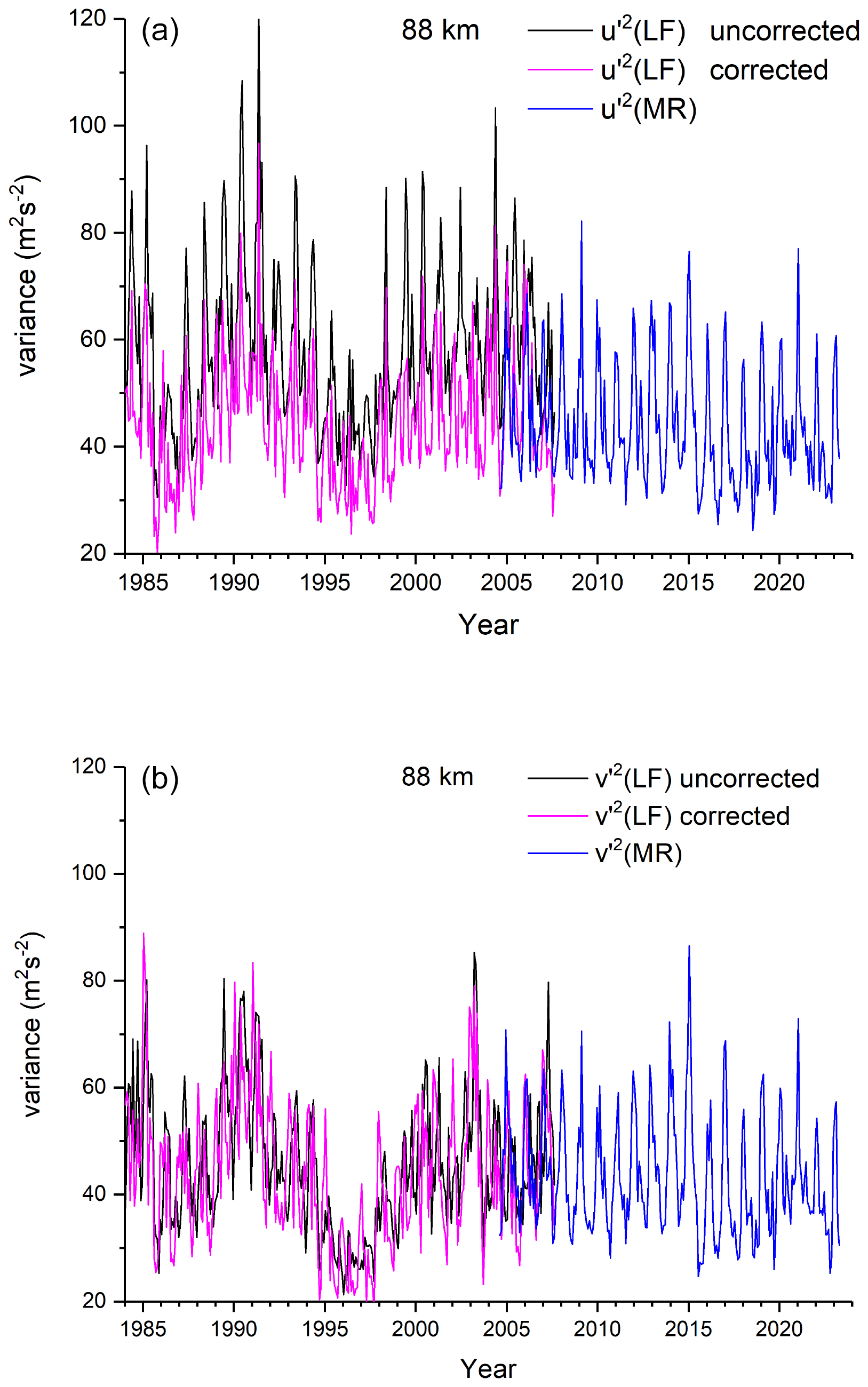
Figure 2 Monthly zonal (a) and meridional (b) variances at 88 km height. Black lines show original LF variances, magenta lines show these after correction.

3 Results

3.1 Seasonal cycle

The long-term mean variance climatology based on the combined LF and MR dataset is shown in Fig. 3. At altitudes above approx. 88 km, the seasonal distribution is dominated by a winter maximum. Minimum values are seen during equinoxes, and a weak secondary summer maximum is visible. At lower altitudes, the summer maximum exceeds the winter one, which at 82 km becomes very weak. This distribution differs from the one shown by Jacobi (2014a) based on LF observations alone. Their results only included the lower part of the height range, and therefore they found the summer maximum, and only a tendency for the winter maximum at higher altitudes. Furthermore, since Jacobi (2014a) did not apply a correction for the zonal-meridional wind bias (Jacobi et al., 2009), their meridional variances especially at greater altitudes became substantially smaller, without a winter maximum.

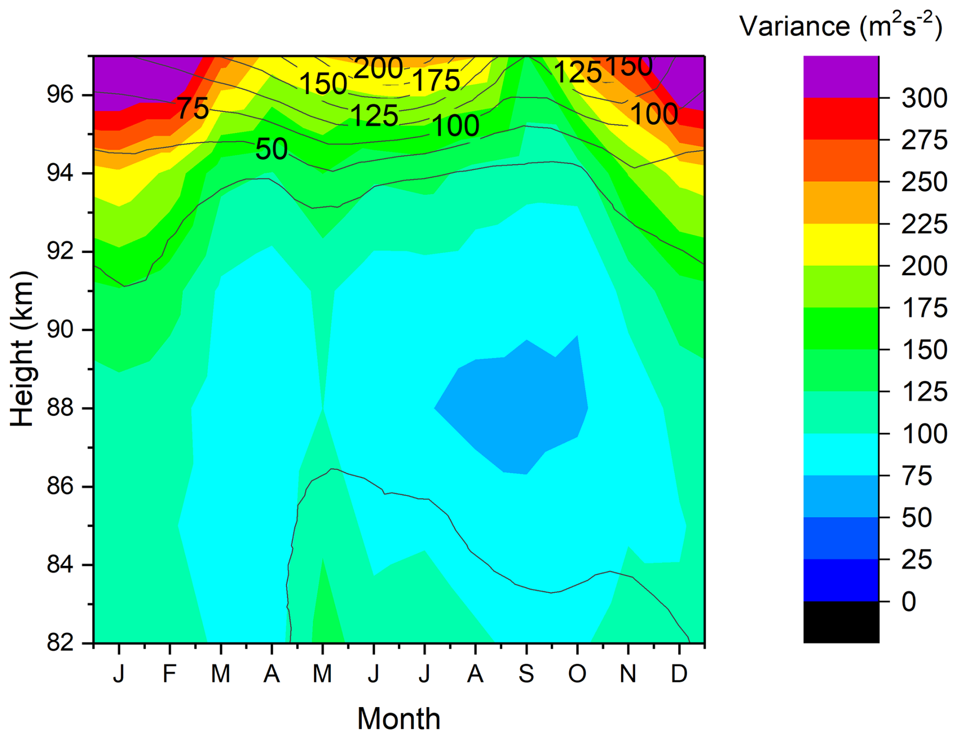
Figure 3 Long-term (January 1984–June 2024) mean total variances ${u^{\prime }}^{\mathrm{2}}+{v^{\prime }}^{\mathrm{2}}$ based on LF and MR observations. Standard deviations based on monthly means are added as black lines.

A winter GW energy maximum has been reported, e.g., by Hoffmann et al. (2011), who also showed a summer maximum and equinox minimum at altitudes around 85 km, as it is seen in Fig. 3. Note that these results referred to a different GW period window and only qualitative agreement can be expected. The same was shown for a single year by Hoffmann et al. (2010). They also presented numerical model results that qualitatively confirmed these results.

3.2 Long-term trends

From earlier LF observations at Collm, Jacobi (2014a) has reported positive GW trends in winter and negative ones in summer. These trends, however, were not very strong, and in most months and height regions not significant, while there was a strong quasi-decadal signature visible, with stronger variance at high solar activity within the 11-year Schwabe cycle. In Fig. 4 we show the seasonal (3-monthly) mean total variances at 88 km in winter (December–February, DJF), spring (March–May, MAM), summer (June–August, JJA) and autumn (September–November, SON). This height gate was chosen because it is closest to the height of maximum meteor rate (e.g., Dawkins et al., 2023). Linear trends based on a least-squares fit are added in the figure. No additional filtering has been applied before the trend estimation. Note that other methods like the Theil–Sen estimator (Theil, 1950; Sen, 1968) are often considered superior to ordinary least-squares, e.g., being insensitive to outliers. Least-squares have been used here to facilitate comparison with earlier analyses, e.g., by Jacobi (2014a). Monthly trend coefficients are shown in Fig. 5. In winter, the trend is slightly positive, while in summer GWs decrease with time. This is qualitatively consistent with the earlier LF results. However, the quasi-decadal cycle visible during the earlier years is strongly reduced since the 2000s. There is also a tendency for a change in phase. While before 2000 GW amplitudes were in phase with solar activity, this appears to be not the case later. We cannot rule out sensitivity especially of the LF observations to solar activity. It is possible that during high solar activity the lower part of the E region is more variable, so that the half-hourly mean height estimates have a larger statistical error than during solar minimum. We cannot check whether this makes an effect on our observations using our dataset alone. But note that the variance minima in the middle of the 1980s and 1990s are consistent with similar minima in the thermosphere as shown by Oliver et al. (2013). Their time series also did not include such minima after the year 2000, which is also consistent with Fig. 4. However, the reason behind the change of decadal variability remains to be explored.

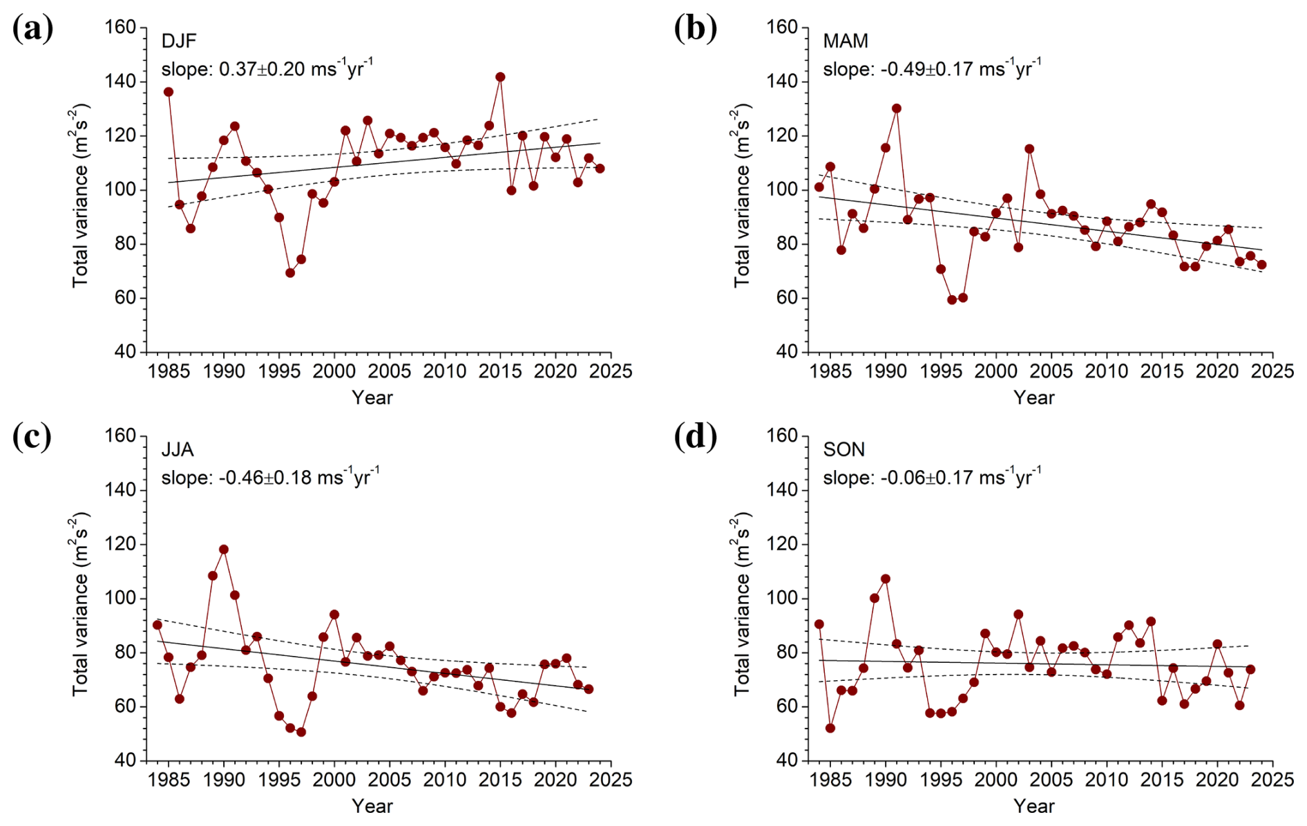
Figure 4 Seasonal mean total variances for (a) DJF, (b) MAM, (c) JJA, and (d) SON over Collm at 88 km altitude. Linear fits are added. Dashed lines show 95 % confidence bands according to a t-test. Trend coefficients and their standard errors are added in the panels.

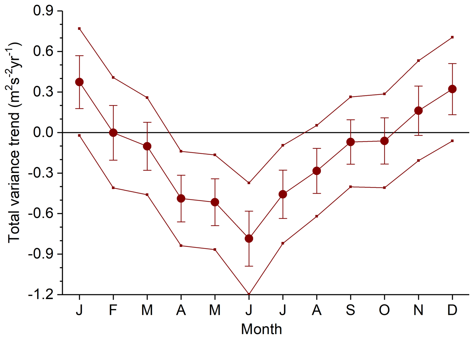
Figure 5 Monthly mean total variances trends at 88 km altitude. Error bars show standard errors. Outer thin lines indicate upper and lower 95 % confidence levels according to a t-test.

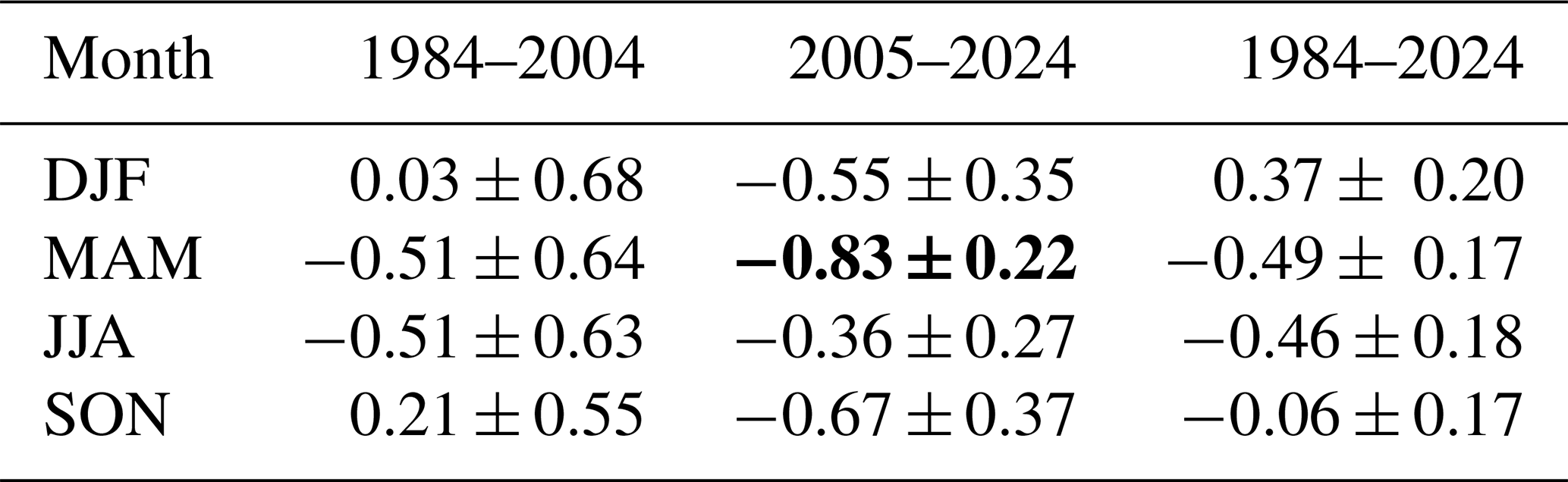
The large variance changes in the 1980s and 1990s lead to low significance levels in trend estimation. It should also be noted that winter trends approximately after the year 2000 are changing and possibly even reversed. In Table 1 the linear trend coefficients for the first (based on LF) and second (based on MR) part of the time series are shown, together with the values for the full series as shown in Fig. 4. The spring and summer trends have the same sign before and after the observational change. The winter trend is negative after 2004, however, fitting the two curves before and after 2005 separately would result in a sudden change in between, so that these trend analyses are not realistic. Due to the shorter time series, the trends are not significant in most cases. In SON, there are insignificant trends that are first positive, then negative. The possible trend changes especially in autumn/winter may be connected with background wind trend changes at that time as it has been noted by Jacobi et al. (2023). A possible reason for this background wind change is ozone recovery after the middle 1990s. Considering MR time series alone, the trend since 2005 is negative in all seasons.

Table 1 Linear trend coefficients (in m s⁻¹ yr⁻¹) for the first part of the time series, the second part, and the full time series. Bold font indicates statistically significant trends at the 95 % level according to a t-test.

The seasonal trends shown in Fig. 4 are consistent with zonal mean wind trends in the mesosphere. Summer and winter mean zonal winds at about 83 km over Juliusruh (about 350 km north of Collm) are shown in Fig. 6. There is a tendency for increasing eastward winds in winter with a trend coefficient and its standard error of 0.09 ± 0.07 m s⁻¹ yr⁻¹, and a decreasing westward (negative) wind trend in summer (slope 0.36 ± 0.15 m s⁻¹) (Jacobi et al., 2023). Note that the summer wind trend is opposite to the trends of maximum mesospheric wind in summer at lower heights of 72–76 km (Jaen et al., 2023). Through wind filtering in the middle atmosphere, GW phase speeds in the upper mesosphere are preferably directed against the wind, so that they propagate westward in winter and eastward in summer. Given a saturated GW, the maximum amplitude equals the intrinsic phase speed, i.e., the difference between mean wind and GW phase speed. Therefore, increasing westerly winter mean winds are connected with increasing GW amplitudes, while decreasing easterly summer winds lead to decreasing GW amplitudes, as shown in Fig. 4.

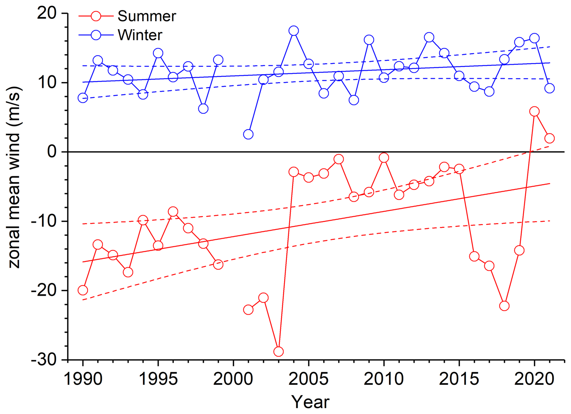
Figure 6 Summer (JJA) and winter (DJF) mean zonal winds at about 83 km over Juliusruh. Dashed lines show 95 % confidence bands according to a t-test from Jacobi et al. (2023).

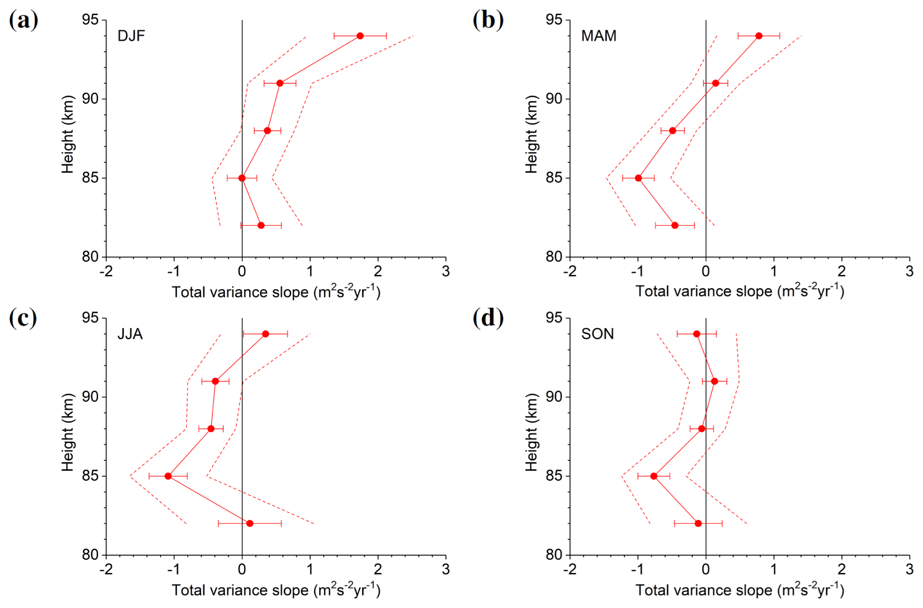
Figure 7 Seasonal mean trend coefficients at 82–95 km altitudes for (a) DJF, (b) MAM, (c) JJA, and (d) SON over Collm. Error bars show standard errors. Dashed lines show upper and lower 95 % confidence levels.

As it has already been shown by Jacobi (2014a), the observed GW trends differ with height. In Fig. 7 we show linear trend coefficients for different seasons and heights. Standard errors and 95 % confidence levels are added. Note that we do not show results for the uppermost level, because due to the sparsity of LF data at that heights there are data gaps even when seasonal means are regarded. In winter, trends are generally positive, but they increase in magnitude with altitude. Partly this is simply due to the GW amplitude increase with height that enhances the absolute values. A similar tendency for the height distribution of trends is visible in spring and summer above 85 km. During these seasons, while in the middle of the considered height interval the trends are negative, they turn towards less negative and even positive values at the lower and upper height gates. Thus, negative trends in summer are consistent with results by Liu et al. (2017), while the positive (although insignificant) trend in summer at 82 km is consistent with the results by Hoffmann et al. (2011). It has to be noted, however, that LF observations are also sparse at lower altitudes, and the trends at 82 km are dominated by the MR data after 2004. A reason for the vertical structure of trends may be a generally positive GW amplitude trend as reported, e.g., by Perminov et al. (2024). During summer, this is superposed by the negative saturation effect described above. During autumn, long-term trends are weaker and, except for the 85 km height gate, not significant.

3.3 Comparison with satellite trends

We analyse SABER GW data for the period 2002–2022 averaged over 30° longitude and 12° latitude over the Collm area. The method how SABER GW data are derived is described, for example, in Ern et al. (2018). We use SABER GW potential energy per volume (E_pot,V) given in J m⁻³. It contains also density and is therefore close to GW momentum flux. If GW horizontal and vertical wavelength do not change, E_pot,V should be a conserved quantity like GW momentum flux. For a discussion see also Strelnikova et al. (2021). Changes of the background wind with altitude, however, will cause Doppler shifts, which in turn would lead to changes in E_pot,V, while GW momentum flux may still be conserved. E_pot,V has the advantage that seasonal variations of atmospheric background density at a fixed altitude are accounted for, and seasonal variations of GW activity and of the background can be better separated. The TIMED satellite performs yaw maneuvres every about 60 d, which means that the SABER latitude coverage changes accordingly. For northward−viewing periods the SABER latitude coverage is about 50° S–82° N, and 82° S–50° N for southward−viewing periods.

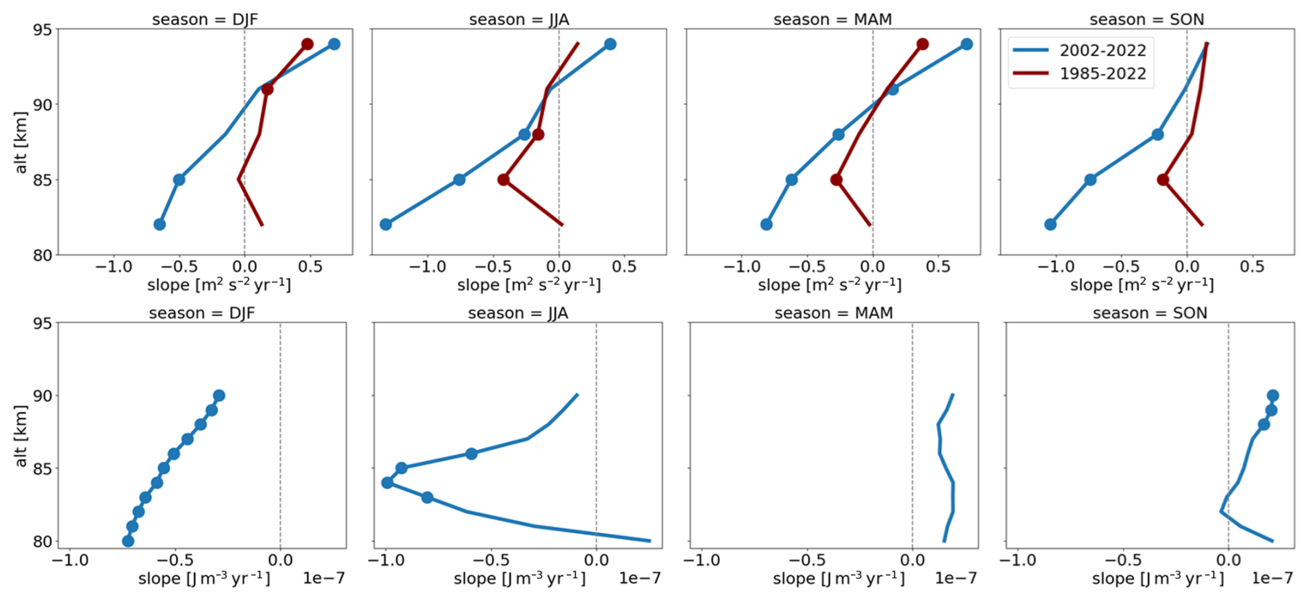
Figure 8 Seasonal mean trends of Collm (upper row) and SABER (lower row) GW proxies with dotted values marked as statistically significant (p-values < 0.05). Dark-red curves refer to the period 1985–2002, while blue curves show data from the period of SABER observations 2002–2022.

Linear trends have been estimated from seasonal means calculated from the preprocessed original data by the Theil–Sen estimator (Theil, 1950; Sen, 1968). The Hamed and Rao Modified Mann-Kendall test (Hamed and Ramachandra Rao, 1998) has been used to assess the significance level (p-value) of our trend estimates to address serial autocorrelation issues. Figure 8 shows trend coefficients of Collm GW proxies in the upper row, while the lower panels show SABER derived E_pot,V trends. At altitudes above 82 km and except for MAM, there is qualitative correspondence of the trends after 2002, and their vertical change. Differences of trends, however, are expected due to the different parameters analysed and the different wavelength ranges seen by radar and satellite. So, horizontal wavelength ranges seen by SABER and MR practically do not overlap (Wright et al., 2016). Discrepancies of trends at the lower levels may also be due to the sparsity of Collm data before 2004. This may also be the reason for the difference of Collm trends with and without the years 1985–2001 (blue and dark-red curves in Fig. 8) at the lower altitude gates. Another source of difference may be the applied averaging of satellite data over 30° longitude and 12° latitude, so that regional effects cannot be excluded.

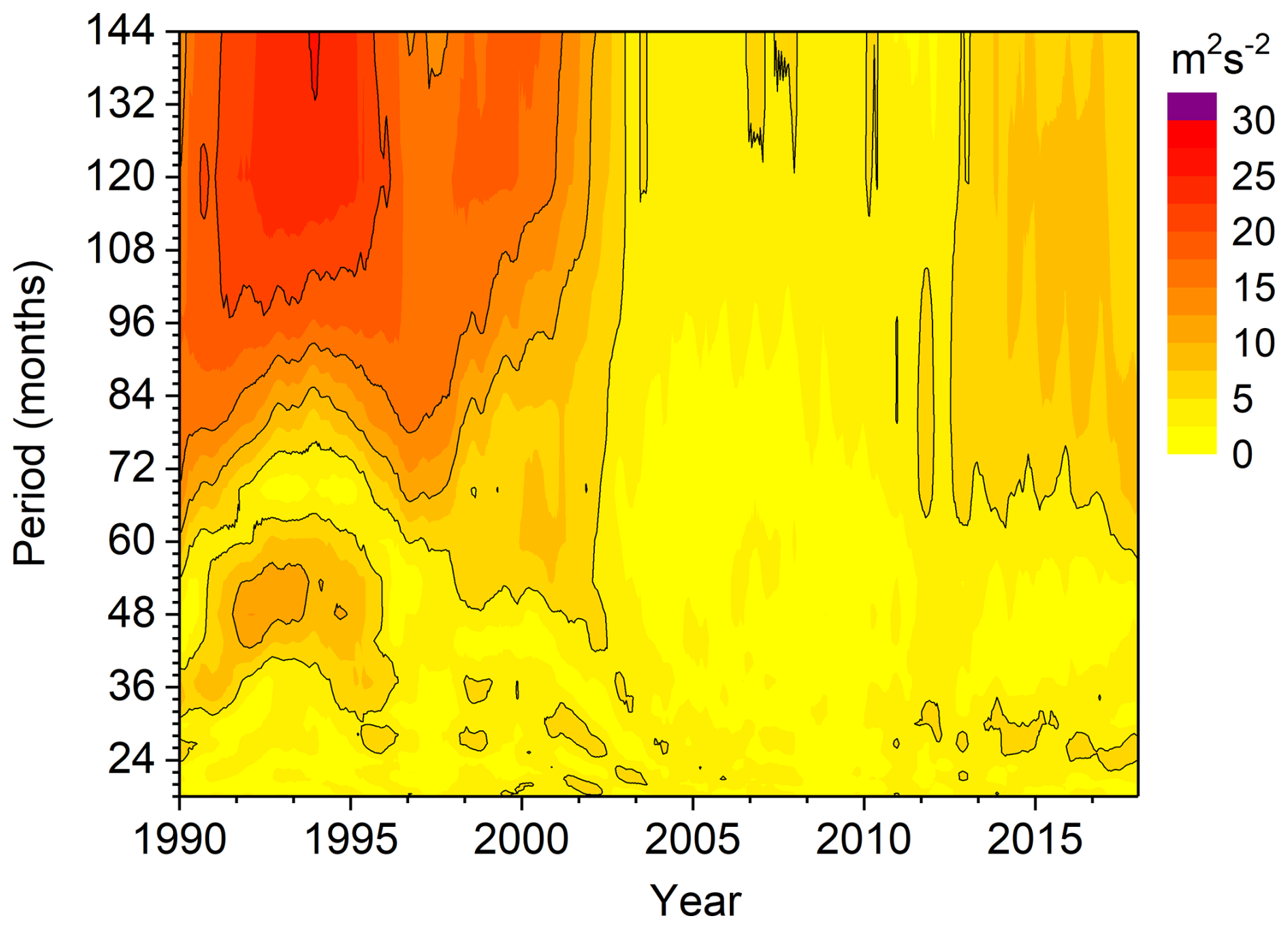
3.4 Interannual variations

We present running periodograms in Fig. 9 based on monthly mean zonal and meridional variances during 12-year data windows each. The figure shows the quasi-decadal variability in the first half of the observations. This signature is seen in each month (see Fig. 4, and partly visible in the mean winds in Fig. 6). In summer, zonal winds minima, related to stronger mesospheric easterly jets are visible around the year 2000 and (weaker expressed) around year 1990. Earlier analyses of Collm mean winds near 90 km based on LF observations show these minima as well (Jacobi and Kürschner, 2006). Stronger mesospheric jets would be consistent with larger GW amplitudes as seen in Fig. 4. In winter, the mean wind decadal oscillation is barely visible, partly, because a positive solar cycle effect on the mean wind in the 1980s and 1990 has been found for autumn, but not for winter (Jacobi and Kürschner, 2006). After the turn of the millennium, this signal vanishes, but later reappeared, although with smaller amplitude. A solar cycle effect on the atmospheric circulation has been found, e.g., by Thejll et al. (2003). We also note interannual variations at the 3–4 year and quasi-biennial time scale. Circulation patterns like El Niño Southern-Oscillation (ENSO) or the Quasi-Biennial Oscillation (QBO) influence the middle atmosphere at mid- to high latitudes at these time scales. Li et al. (2016) proposed that warm ENSO events cause anomalous Southern Hemisphere stratospheric easterly zonal wind and the resulting perturbation to GW filtering causes anomalous mesospheric eastward GW forcing. ENSO signatures are visible throughout the stratosphere and mesosphere, but in the MLT the signal may depend on the considered time interval and the height (Jacobi et al., 2017; Ermakova et al., 2019). This may be a reason for the intermittent signature on 3–4 year signals in Fig. 9.

Figure 9 Running periodograms of total variance based on monthly data at 88 km altitude.

4 Conclusions

We have shown wind variances calculated from half-hourly wind differences in MLT observations by two different methods, namely the LF spaced received method and observations by MR. We have applied a bias correction and thus were able to present monthly means in an altitude range from 82 to 97 km and time series from 1984 to 2024. The long-term mean variances exhibit a winter maximum, and a secondary summer maximum especially visible in the upper mesosphere and less clearly in the lower thermosphere. This distribution is qualitatively consistent with earlier observations and model results (Hoffmann et al., 2010, 2011).

GW activity in the MLT changes with time. In the lower thermosphere, during most seasons a positive trend is visible, consistent with literature results (Oliver et al., 2013; Perminov et al., 2024). In the summer MLT, trends are mostly negative, while in the upper mesosphere there is a tendency for positive trends again. The latter is consistent with other reported trends (Hoffmann et al., 2011), but our results at 82 km are not statistically significant. Comparison with satellite-derived GW potential energy trends showed qualitative correspondence, but not at all altitudes and each season. One of the reasons for discrepancies might be different wavelength ranges observed by the MR and satellite systems.

GW amplitudes vary at different time scales. In particular, there is a quasi-decadal oscillation, which is strongly expressed during the first half of our time series, but then vanishes and reappears later with smaller amplitude. This is qualitatively consistent with results by Oliver et al. (2013). We also observe intermittent interannual variations at time scales of 2–4 years.

Long-term trends, decadal, and interannual changes of GW activity in the MLT may be a signature of GW-mean flow coupling in the middle atmosphere. Future analyses therefore should combine mean wind and GW observations, preferably also at lower altitudes in the mesosphere. For this, partial reflection radars such as the Juliusruh one (e.g., Jaen et al., 2022, 2023) could be employed.

Appendix A: Bias correction table

Table A1 LF $/$ MR ratios for zonal and meridional variances, for each month of the year and each height gate, based on overlapping measurements from August 2004 to August 2007.​​​​​​​​​​​​​​