Measurement Uncertainty of Radiated Electromagnetic Emissions in In Situ Tests of Wind Energy Conversion Systems

The electromagnetic (EM) emissions of wind energy conversion systems (WECS) are evaluated in situ. Results of in situ tests, however, are only valid for the examined equipment under test (EUT) and cannot be applied to series production as samples, as the measurement uncertainty for in situ environment is not characterized. Currently measurements must be performed on each WECS separately, this is associated with significant costs and time requirement to complete. Therefore, in this work, based on the standard procedure according to the “Guide to the Expression of Uncertainty” (GUM, 2008) the measurement uncertainty is characterized. From current normative situation obtained influences on the measurement uncertainty: wind velocity and undefined ground are evaluated. The influence of increased wind velocity on the measurement uncertainty is evaluated with an analytical approach making use of the dipole characteristic. A numerically evaluated model provides information about the expected uncertainty due to reflection on different textures and varying values of relative ground moisture. Using a classical reflection law based approach, the simulation results are validated. Thanks to the presented methods, it is possible to successfully characterize the measurement uncertainty of in situ measurements of WECS's EM emissions.

1 Introduction and Motivation

In order to meet the goal of the 2015 Paris agreement, it is necessary to reduce the amount of carbon dioxide emissions currently being produced (UNFCC, 2015). The reduction of carbon dioxide emissions is a movement towards power generation systems with renewable energy sources instead of fossil ones. One approach is to operate wind energy conversion systems (WECS). Like all other industrial, scientific and medical (ISM) devices, WECS must be assessed and evaluated regarding their radiated electromagnetic (EM) emissions based on international standards (CISPR 11, 2015). Due to their geometrical size, WECS cannot simply be installed and tested at a defined test site such as an open area test site (OATS). Instead, they need to be tested in situ. The problem is, that for equipment under test (EUT), evaluated in situ only, compliance with these standards can be proven for this specific EUT, but not for the whole product line. In order to reduce the effort and costs, it is always aimed for a series release. However, a series release is only possible with the knowledge of the measurement uncertainty, determined according to the “Guide to the Expression of Uncertainty in Measurement” (GUM, 2008). The measurement uncertainty for in situ tests of WECS is not specified yet. Therefore, the goal of this work is to define and characterize possible contributions to uncertainty during in situ measurements of EM emissions from WECS. The normatively given limit values as well as the causes of the EM emissions are not focus of this article. The latter are discussed e.g. in Koj et al. (2017) and Fisahn et al. (2017).

This paper explains the measurement of EM emissions of WECS according to the normative situation in the second Chapter. Subsequently, Sect. 3 describes the standard procedure for the determination of the measurement uncertainty according to GUM. In Sect. 4 the normative situation on determination of the uncertainty in EM emission tests is analysed. The comparison between OATS and in situ leads to two main emphases: the deflection of the antenna due to wind velocity and the reflection of EM waves on different grounds. The numerical and analytical evaluation of the antenna deflection is presented in Sect. 5 and the influence of the ground reflections is discussed in Sect. 6 respectively. A conclusion of the significant results completes this article.

2 In Situ Measurements on WECS

In this chapter the determination of the EM emissions of WECS according to the normative situation is roughly sketched. Further, more detailed considerations on this topic can be found in e.g. Koj et al. (2016a, b).

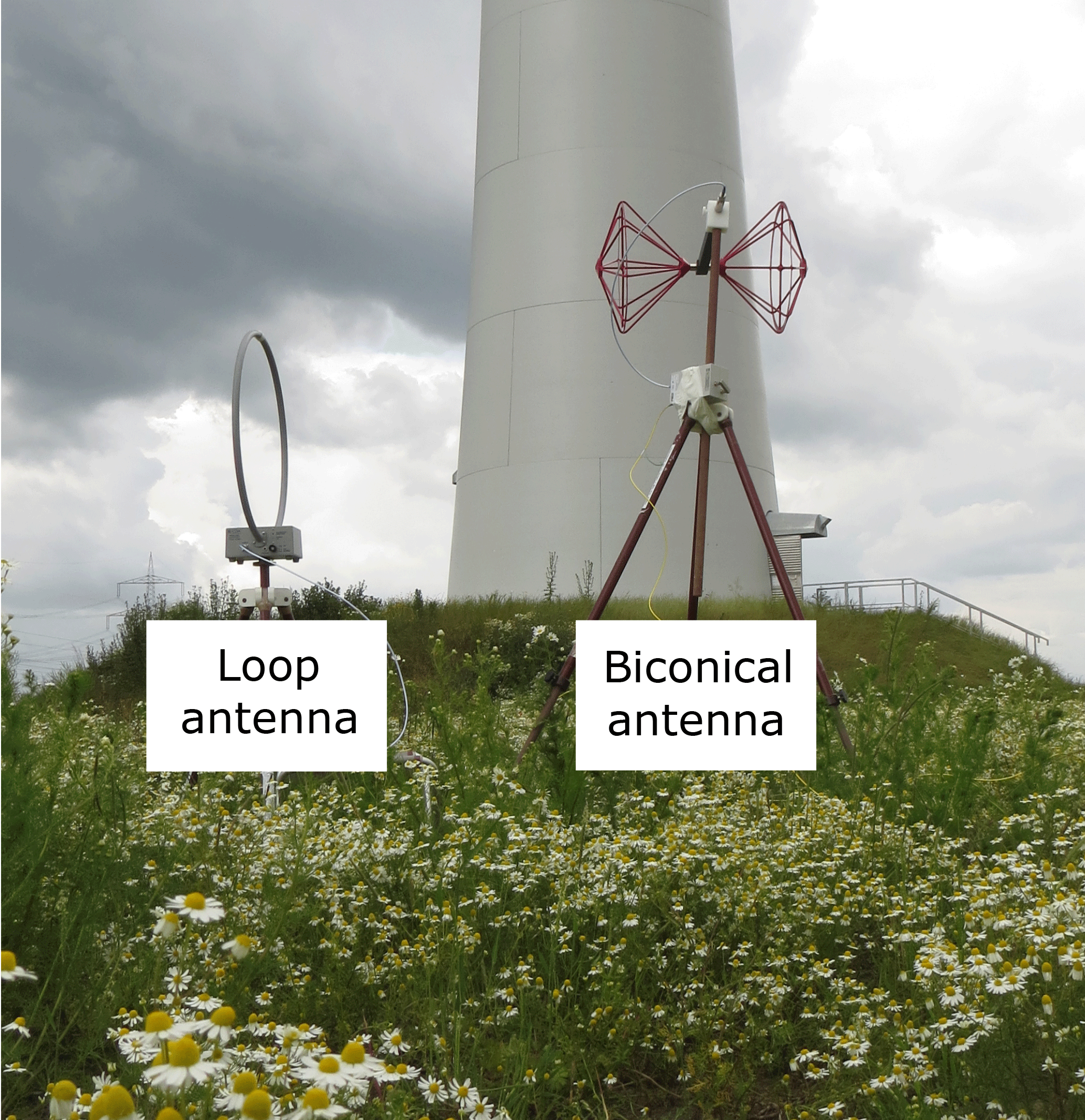
WECS, also known as wind turbines (WTs), have to be evaluated with respect to their radio frequency (RF) disturbances respectively as well as the radiated emissions from other ISM (industrial, scientific and medical) electrical and electronic equipment. Therefore, the proof of compliance according to the Directive 2014/30/EU with the national implementation of this directive (e.g. the EMC Law, 2016 in Germany), must be provided. The standard CISPR 11 deals with the measurement methods and limits for the RF disturbances of ISM equipment. With respect to this standard, WTs must be classified into Group 1 and Class A, since the WT forms an unintentional radiator (Group 1) that is always located and operated out of living areas (Class A). Because of the enormous geometrical dimensions of a WT with a typical height of more than 100 m, the only practical way to assess the device is to perform an in situ measurement, even though equipment that is classified into Group 1 could be tested either on a test site or in situ. Thus, the radiated emissions have to be determined solitarily in order to be evaluated. Therefore, the emission measurements have to be carried out with an antenna and an EMI receiver according to CISPR 16-1-1 (2015), CISPR 16-1-4 (2010), CISPR 16-2-3 (2010), CISPR 16-4-2 (2011) and CISPR/TR 16-2-5 (2008) so as to measure the magnetic field strength in the frequency range from 150 kHz to 30 MHz (CISPR Band B) respectively the electric field strength in the range from 30 MHz to 1 GHz. The latter frequency range corresponds to the CISPR Bands C (30–300 MHz) and D (300 MHz–1 GHz). Figure 1 shows examples of standard compliant antennas. Using the loop antenna, the recorded magnetic field strength and the biconical antenna, the electric field strength can be measured. The above mentioned standards also allow the use of a logarithmic periodic dipole antenna (LPDA) for the electric field strength measurement, whereby both polarizations of the electric field strength shall be measured, the horizontal and the vertical.

Figure 1 Example antennas for measuring the radiated RF emissions of wind turbines.

Further information about a measurement campaign at a WT can be found in the technical guideline FGW/TR 9, 2014. This guideline describes the procedure for the uniform definition of measuring positions, where the RF emissions shall be measured. An example of this is shown in Fig. 2. The field measurements must be carried out on at least four measuring positions, whereby the distance between the outer tower wall and the measuring position should be 30 m each. In order to ensure the reproducibility of the measuring positions, there should be a fixed reference point chosen, e. g. the tower door of the WT. At each of the measuring positions, the WT must be measured in at least two modes: when the WT is in power harvesting mode, and when the WT is turned off. Further modes can be found in the FGW/TR 9. The measured field strength values of each measuring position should be rated using the limit values given by CISPR 11. If the measured radiated emissions are below these frequency dependent limits, the wind turbine will pass the test, otherwise it will fail.

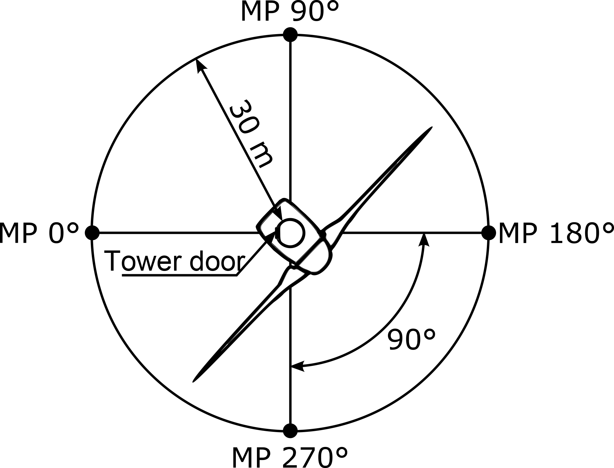
Figure 2 Top view on a wind turbine (WT). The measuring positions (MP) are located around the WT (FGW/TR 9, 2014). The tower door sets the orientation of the reference frame.

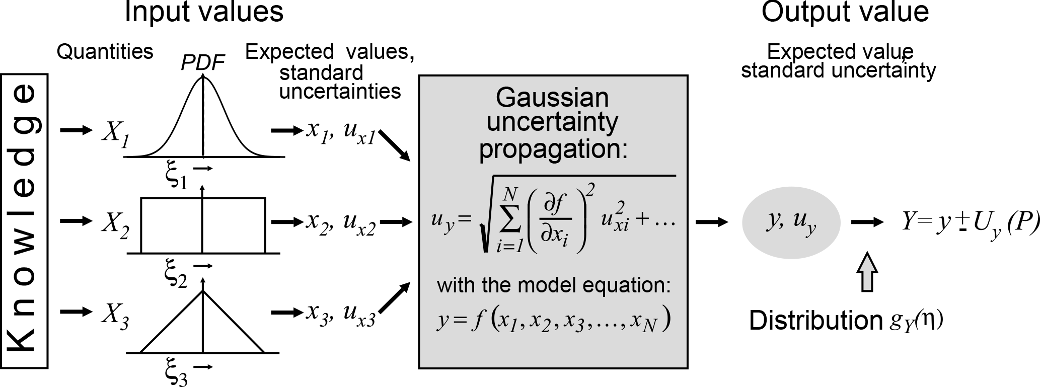
Figure 3 Procedure for determining the measurement uncertainty according to GUM (Sommer and Siebert, 2004).

A general explanation of the uncertainty of measurement will be discussed in the following chapter.

3 Determining the Measurement Uncertainty According to GUM

A measurement result is only complete with inclusion of the associated measurement uncertainty. In order to determine the measurement uncertainty, the method according to GUM, which has been established in recent years, is utilized. This method is described in detail in various publications, for example in Sommer and Siebert (2004). Therefore, in this chapter, the standard GUM procedure is only succinctly explained. The procedure requires a model equation for the measurand Y:

$$\begin{array}{}\text{(1)}& Y=f(X_{\mathrm{1}},X_{\mathrm{2}},\mathrm{\dots },X_N).\end{array}$$

The measurand Y, also referred to as output value shown in Fig. 3, is dependent on input values X_i, with $i=\mathit{\{}\mathrm{1},\mathrm{2},\mathrm{\dots },N$, such as the quantities as well as the probability density function (PDF).

In most cases it is not possible to specify the input values exactly. With knowledge of the limitation of the possible input values ξ_i of X_i and with the associated PDF, the input values can be characterized by their expected values

$$\begin{array}{}\text{(2)}& x_i=E\left[X_i\right]\end{array}$$

and standard uncertainties

$$\begin{array}{}\text{(3)}& u_{xi}=\mathit{\{}E\left[{\left(X_i-x_i\right)}^{\mathrm{2}}\right]{\mathit{\}}}^{\mathrm{1}/\mathrm{2}}.\end{array}$$

Using the Gaussian uncertainty propagation, the output value Y can be characterized by the expected value

$$\begin{array}{}\text{(4)}& y=E\left[Y\right]=f(x_{\mathrm{1}},x_{\mathrm{2}},\mathrm{\dots },x_N)\end{array}$$

and the associated standard uncertainty

$$\begin{array}{ll}{\displaystyle }& {\displaystyle }{u}_y={\left\{\sum _{i=\mathrm{1}}^N{\left({\displaystyle \frac{\partial f}{\partial x_i}}\right)}^{\mathrm{2}}{u}_{xi}^{\mathrm{2}}+\mathrm{2}\sum _{i=\mathrm{1}}^{N-\mathrm{1}}\sum _{j=i+\mathrm{1}}^N{\displaystyle \frac{\partial f}{\partial x_i}}{\displaystyle \frac{\partial f}{\partial x_j}}{u}_{xixj}\right\}}^{\mathrm{1}/\mathrm{2}}\\ \text{(5)}& {\displaystyle }& {\displaystyle }={\left\{\sum _{i=\mathrm{1}}^N{c}_i^{\mathrm{2}}{u}_{xi}^{\mathrm{2}}+\mathrm{2}\sum _{i=\mathrm{1}}^{N-\mathrm{1}}\sum _{j=i+\mathrm{1}}^N{c}_i{c}_j{u}_{xixj}\right\}}^{\mathrm{1}/\mathrm{2}}\end{array}$$

where $u_{xixj}=u_{xi}\cdot u_{xj}\cdot r\left(x_i;x_j\right)$ is estimated covariance associated with x_i and x_j and r(x_i;x_j) is the correlation coefficient.

For a complete measurement result $Y=y\pm U_y\left(P\right)$, the expanded measurement uncertainty $U_y\left(P\right)=k_p\cdot u_y$ is required. U_y(P) indicates the interval in which the value of the measurand is located with a probability P. The coverage factor k_p depends on the PDF of the output value Y. Usually, a normal PDF, a probability P=95 % and thus k_p=2 is assumed.

This work focuses in the definition and on the characterization of the input values according to Fig. 3. For this purpose, the following chapter considers the normative situation for measurement uncertainty in other test sites.

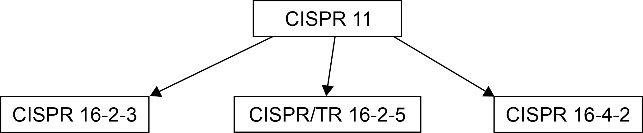
Figure 4 Overview of standards with information on measurement uncertainty in EM emission measurements.

4 Challenges in Determining the Measurement Uncertainty in In Situ Tests of WECS

As shown in Fig. 4, CISPR 11 refers to the CISPR 16-2-3, CISPR/TR 16-2-5 and CISPR 16-4-2 standards in terms of measurement uncertainty. CISPR 16-2-3 contains general advice about performance of measurement campaign. In the annexes informations and specifications for measurements in the presence of environmental interferences can be found. While CISPR/TR 16-2-5 defines requirements to in situ measurement in general, of interest is in particular the demand to carry out in situ measurement campaign at wind velocities below 10 m s⁻¹ and in “dry weather”. Finally, CISPR 16-4-2 establishes terms of references on uncertainty in measurements of EM emissions for various test environments, except in situ. Comparing in situ to other test sites covered in the CISPR 16-4-2, it can be said that the OATS is most similar to the in situ environment. The terms of reference in CISPR 16-4-2 contain the model equation for determining the field strength (measurand) and standard uncertainties of the input values, which can be divided into three groups:

1. Measuring equipment,

2. Test setup,

3. Measurement environment.

The “measuring equipment” (receiver display, antenna factor) used on OATS and in situ is the same, thus all input values are conform and can be adopted to in situ measurement.

For the category “test setup” the influence of the wind velocity has to be investigated (the other measurement uncertainty aspects can be adopted). The requirement of the CISPR/TR 16 2-5 to carry out the measurements at wind velocity below 10 m s⁻¹ is of no use evaluating WECS, because usually their rated power is reached at this wind velocity. The author's experience of various measurement campaigns is, that higher wind velocities causes deflection of the antenna tripod. Therefore, the resulting standard uncertainty is evaluated in Sect. 5.

The category “measurement environment” shows the biggest differences between the OATS and in situ environment. OATS should be placed (theoretically) far away from sources of interference and the ground should be (perfectly) conductive in order to enable reproducible measurement results. In contrast, WECS are often installed in industrial environments, where the presence of other sources of interference must be expected. Furthermore, the electromagnetic properties of the soil around a WT depends on the local texture (clay, sand) and also varies in time due to weather conditions (moisture). In order to deal with environmental EM disturbances in the vicinity of WECS, the instructions of CISPR 16-2-3 can be consulted. Approaches to deal with uncertainties due to undefined ground conditions around a WT are presented in Sect. 6.

5 Contribution of the Wind Velocity to the Measurement Uncertainty

The impact of wind velocity on the measurement uncertainty is evaluated in two steps. First, numerical simulations and an analytical approach relate the antenna deflection with the field deviation. Second, the wind related uncertainty is estimated relating measurement deviation and the wind velocity.

5.1 Antenna Deflection and Corresponding Deviation

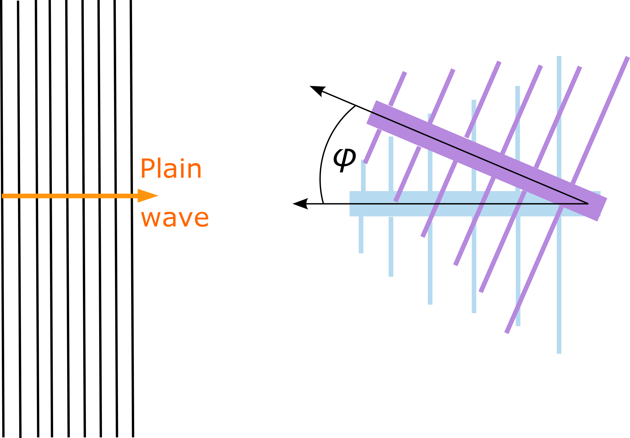
Taking into account the CISPR 11 Bands the evaluation is divided in three parts: Band B, C and D. As CISPR 16-2-3 instructs to use a loop antenna to measure the magnetic field component at a height h₁=1 m above ground (in Band B), no relevant deflection of the tripod can be observed during measuring campaigns using a standard tripod. The electric field has to be measured according to CISPR 16-2-3 at a height h₂=2 m above ground using a biconical antenna for measurements in Band C and a LPDA for measurements in Band D. Due to the height and larger wind exposed areas of the electrical antennas, their deflection of approx. φ=7^∘ on a standard tripod can be observed during both polarization measurements, horizontal and vertical. To evaluate this impact on the results simulations with the field simulator for radio emission problems “Concept II” are set-up. For the CISPR Band C a biconical antenna is modeled and for the CISPR Band D ten adapted dipoles are modeled in the CAD tool provided by ”Concept II”. In the simulation those antennas are tilted in a plain wave field as shown in Fig. 5 (here for an LPDA) while feed point voltage is detected. In order to calculate the deviation

$$\begin{array}{}\text{(6)}& D_{\mathrm{W}}=\mathrm{20}\log \left({\displaystyle \frac{U_{\mathit{\phi }}}{U_{\mathrm{0}}}}\right)\end{array}$$

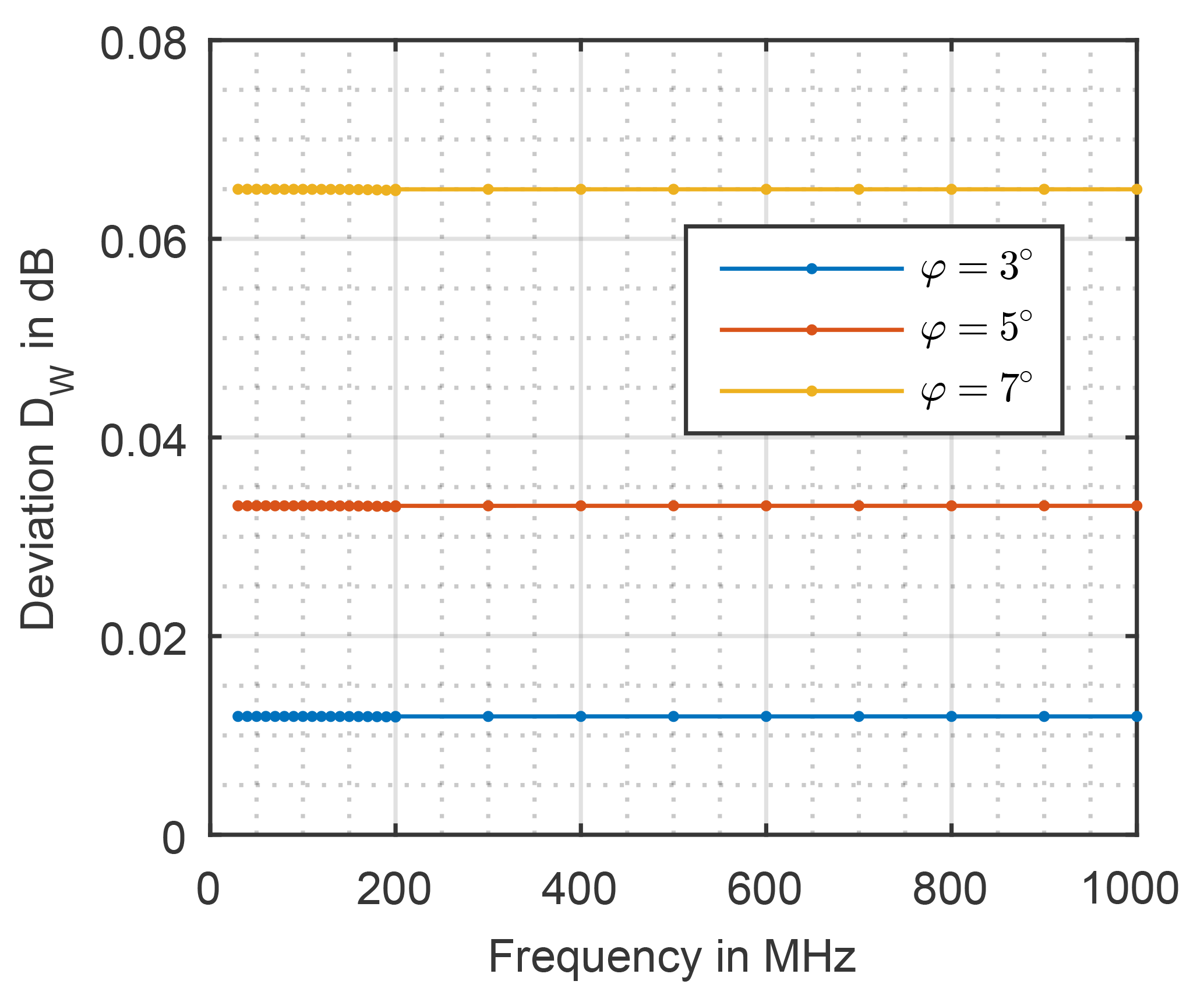
the feed point voltage of the tilted antenna U_φ is divided by the feed point voltage U₀ at tilting angle of zero. As shown in Fig. 7 the deviation at each angle is constant over the frequency spectrum. Furthermore, it can be seen that same deviation occurs at the same angle for both, the biconical antenna and LPDA.

Figure 5 Tilted LPDA in plain wave field.

Figure 6 Dipole characteristic. φ is the deflection angle.

Figure 7 Simulated deviation of feed point voltage for different antenna tilting angles.

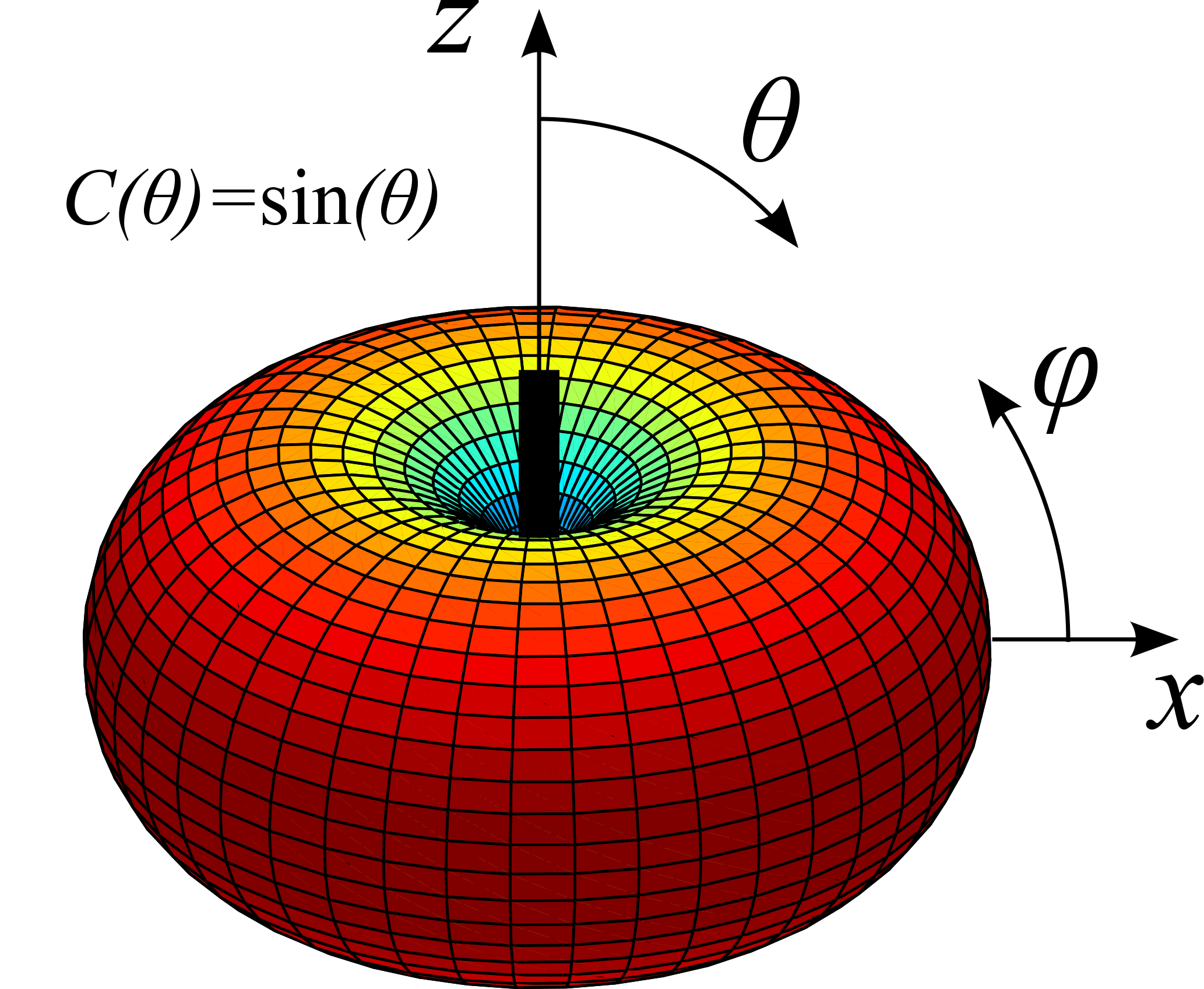
By approximating the behavior of the antennas by an adapted dipole of which the directional pattern has a well-known torus geometry C(θ) = sin (θ) (Balanis, 2005), shown in Fig. 6, the deviation D_W can be calculated with

$$\begin{array}{}\text{(7)}& D_{\mathrm{W}}=\mathrm{20}\left|\log \left({\displaystyle \frac{\sin (\mathrm{|}\mathrm{90}{}^{\circ }-\mathit{\phi }\mathrm{|})}{\sin \left(\mathrm{90}{}^{\circ }\right)}}\right)\right|=\mathrm{20}\mathrm{|}\log \left(\cos \right(\mathit{\phi }\left)\right)\mathrm{|}\end{array}$$

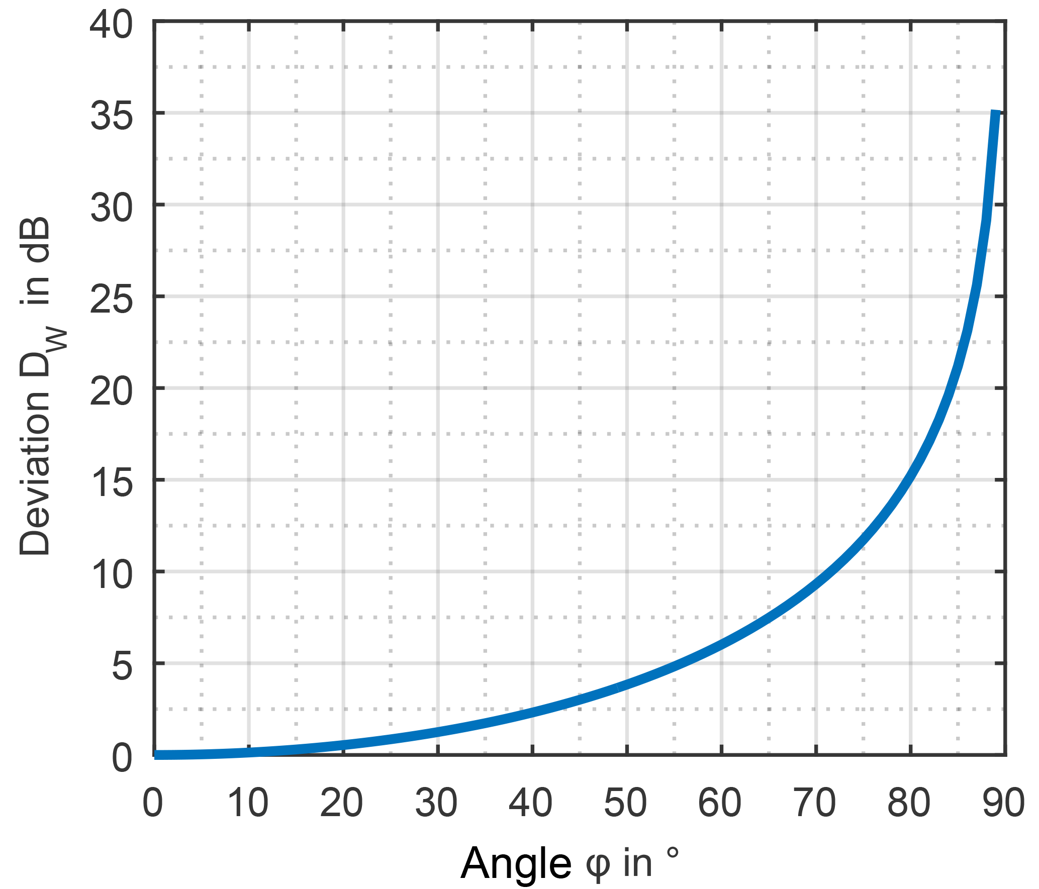
The deviation derived from simulation and the deviation evaluated analytically are equivalent and plotted in Fig. 8 over the tilting angle. Thanks to the dipole characteristic, the deviation can be described analytically by Eq. (7). In a next step, the relation between the wind velocity and the wind related deviation will be deduced.

Figure 8 Analytically calculated deviation over the tilting angle of the dipole.

Figure 9 Antenna tripod modelled as a bending beam strained by wind force F_W.

5.2 Realistic Wind Velocities and Standard Uncertainty

The tilting angle of the antenna is caused by the deflection of the tripod due to wind force, therefore the tripod is modeled as a bending beam, shown in Fig. 9. In order to evaluate the deviation of antenna directivity by wind velocity the tilting angle is related to the wind force F_W by

$$\begin{array}{}\text{(8)}& \mathit{\phi }=\arctan {\displaystyle \frac{F_{\mathrm{W}}{l}^{\mathrm{2}}}{\mathrm{6}EI}}\end{array}$$

where l is antenna tripod height, E is the modulus of elasticity and I is the tripod inertia (Gross et al., 2005).

The following Eq. (9)

$$\begin{array}{}\text{(9)}& F_{\mathrm{W}}=A_{\mathrm{S}}{c}_{\mathrm{p}}{\displaystyle \frac{\mathit{\rho }}{\mathrm{2}}}{v}^{\mathrm{2}}\end{array}$$

relates the wind force F_W and the wind velocity v, where A_S is wind-exposed area, c_p is the pressure coefficient and ρ is the atmospheric pressure (Blohm, 1975).

By inserting Eqs. (8) and (9) in Eq. (7) and taking into account the parameters of a typical wooden antenna tripod, the wind caused deviation D_W can be given as a function of wind velocity. According to FGW/TR 9, WECS are operating at wind velocities between 3 and 27 m s⁻¹ what leads to maximum deviation $D_{\mathrm{W},\max }=\mathrm{0.06}$ dB, as shown in Fig. 10. Hence, the standard uncertainty u_W caused by wind velocity can be calculated assuming a rectangular distribution between 0 and 0.6 dB with

$$\begin{array}{}\text{(10)}& u_{\mathrm{W}}={\displaystyle \frac{D_{\mathrm{W}}\left(\mathrm{27}\mathrm{m}{\mathrm{s}}^{-\mathrm{1}}\right)}{\mathrm{2}\sqrt{\mathrm{3}}}}=\mathrm{0.02}\mathrm{dB}\end{array}$$

In this way, the wind velocity related standard measurement uncertainty can be characterized. The analysis of the presented mechanical antenna model is based on the assumption that the antenna structure is in a homogeneous and laminar wind field. Thus, the resulting uncertainty is assumed for both, the horizontal and the vertical orientation of the electrical antenna. In the next chapter the uncertainty of field reflection on undefined ground is considered.

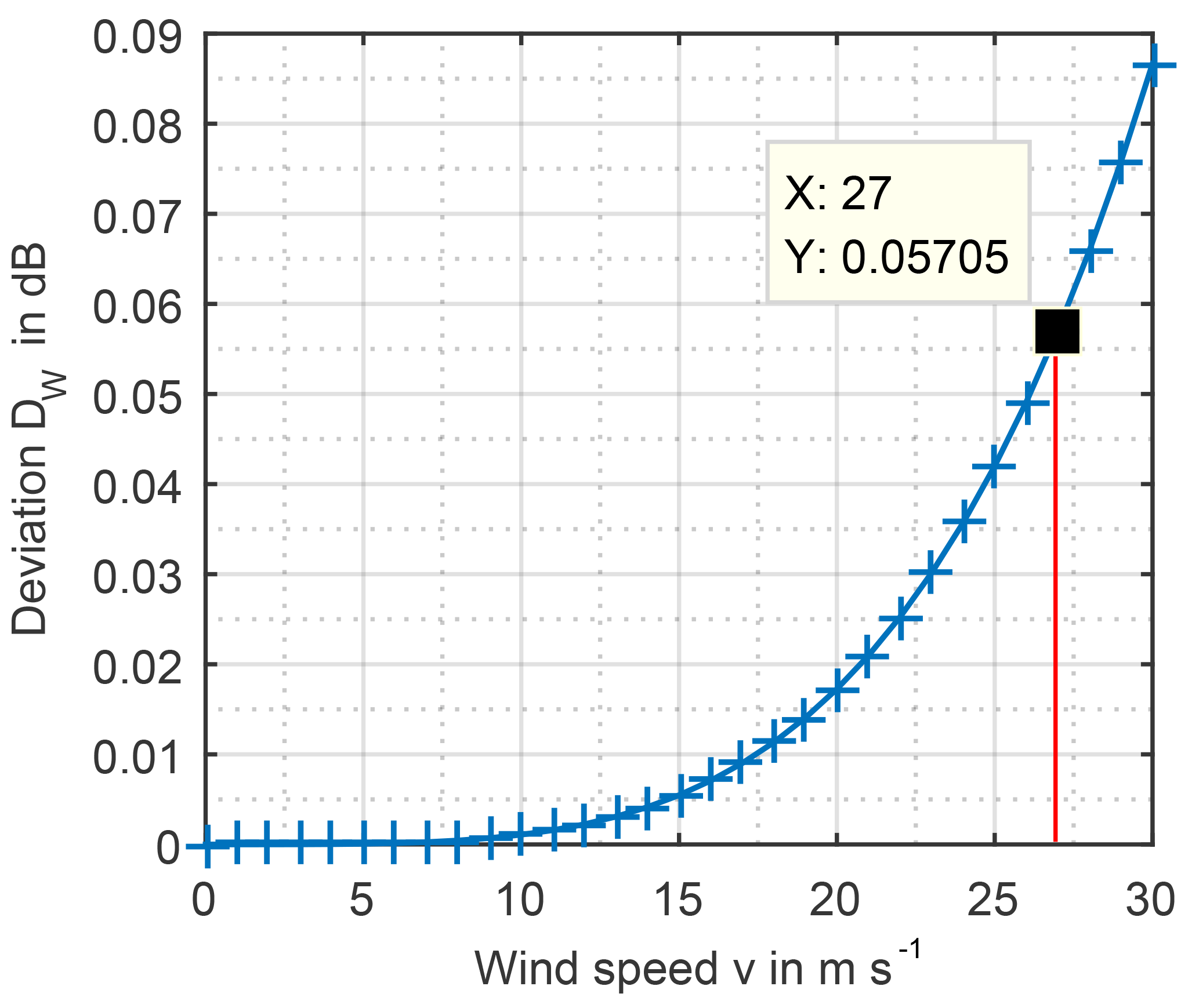
Figure 10 Analytically calculated deviation over the wind velocity. At wind velocity of 27 m s⁻¹, WECs are turned off.

6 Influence of the Ground on the Measurement Uncertainty

The evaluation of the reflected EM field on undefined ground is approached in two ways. A numerical one – explained in Sect. 6.1 – uses a simplified model of a WT to calculate the EM fields above the ground. The ground properties are simulated by varying EM parameters of electrical conductivity and relative permittivity. And a conservative one – explained in Sect. 6.2 – known from the law of reflection. The grounds chosen are electrically neutral (free space) and PEC. The obtained standard uncertainty follows a worst case scenario, thus used for validation of the simulation results.

6.1 Numerical Simulation

Of all the possible grounds WECS can be built on, sand has the lowest conductivity while clay has the highest; therefore, those textures are considered the two extremes (Hippel, 1995). In order to evaluate the reflection of WT's EM emission on undefined ground a simulation is set-up in FEKO, a field simulator by Altair. As shown in Fig. 11, a l=100 m long bottom loaded monopole, approximating a WT, is placed above an infinitive extended ground.

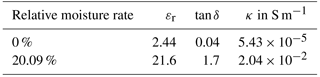
The ground relative permittivity ε_r and conductivity κ meets with either sand or clay with varying moisture rate. The frequency depended values are taken from Hippel (1995). As an example, the values for 10 MHz are shown in Table 1.

Figure 11 Bottom loaded monopole as a simplified model of a WT.

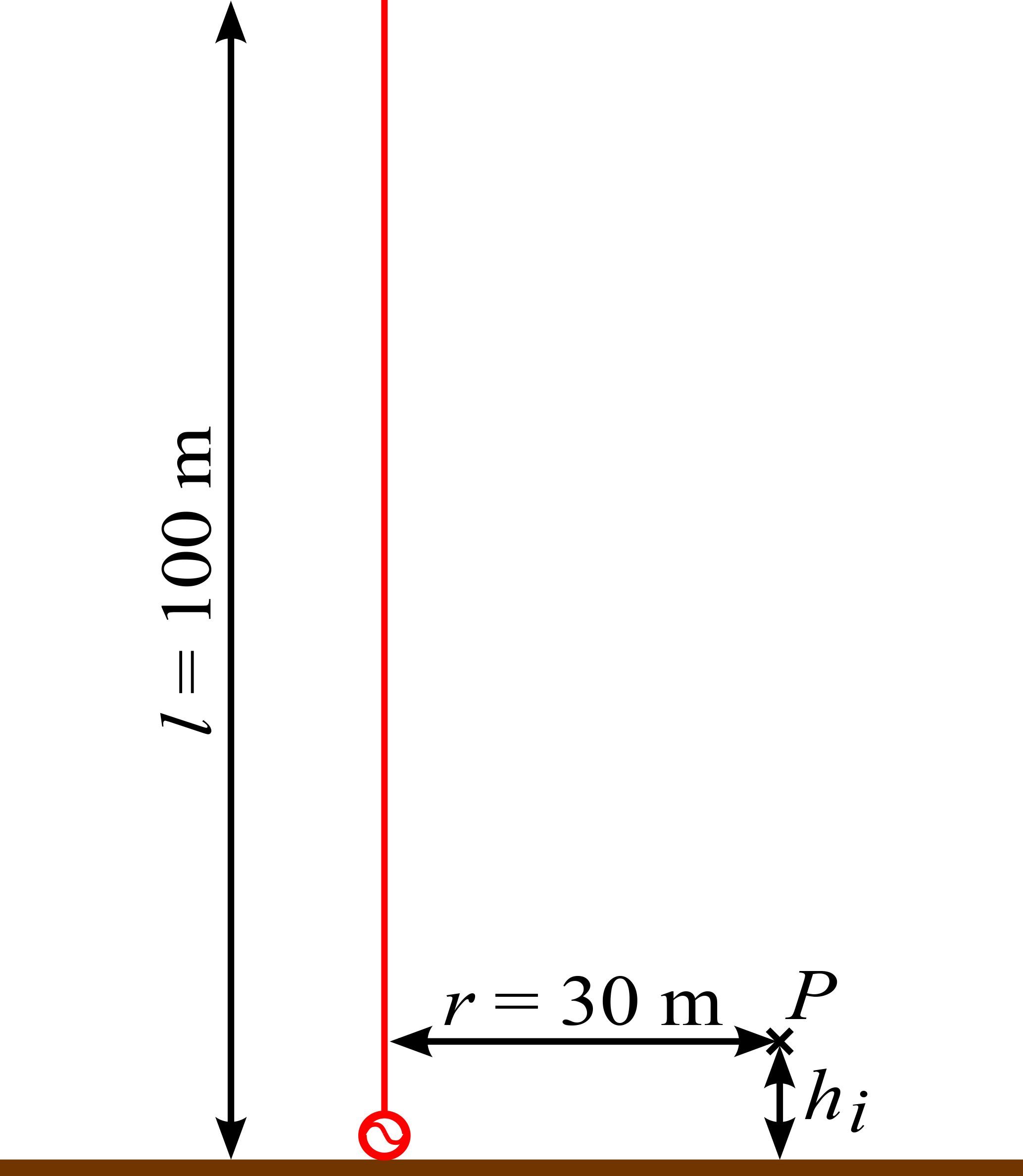
Table 1 Exemplary parameters for clay at 10 MHz (Hippel, 1995).

Carrying out the simulation the field is detected corresponding to CISPR 16-2-3 in r=30 m distance and h₂=2 m above the ground (Fig. 11). In order to validate the model, the simulation is run in free space and with perfect electric conducting (PEC) ground. The field strength with PEC is for the entire spectrum lower than the doubled field strength in free space, as shown in Fig. 12. Thus, the model can be assumed correct.

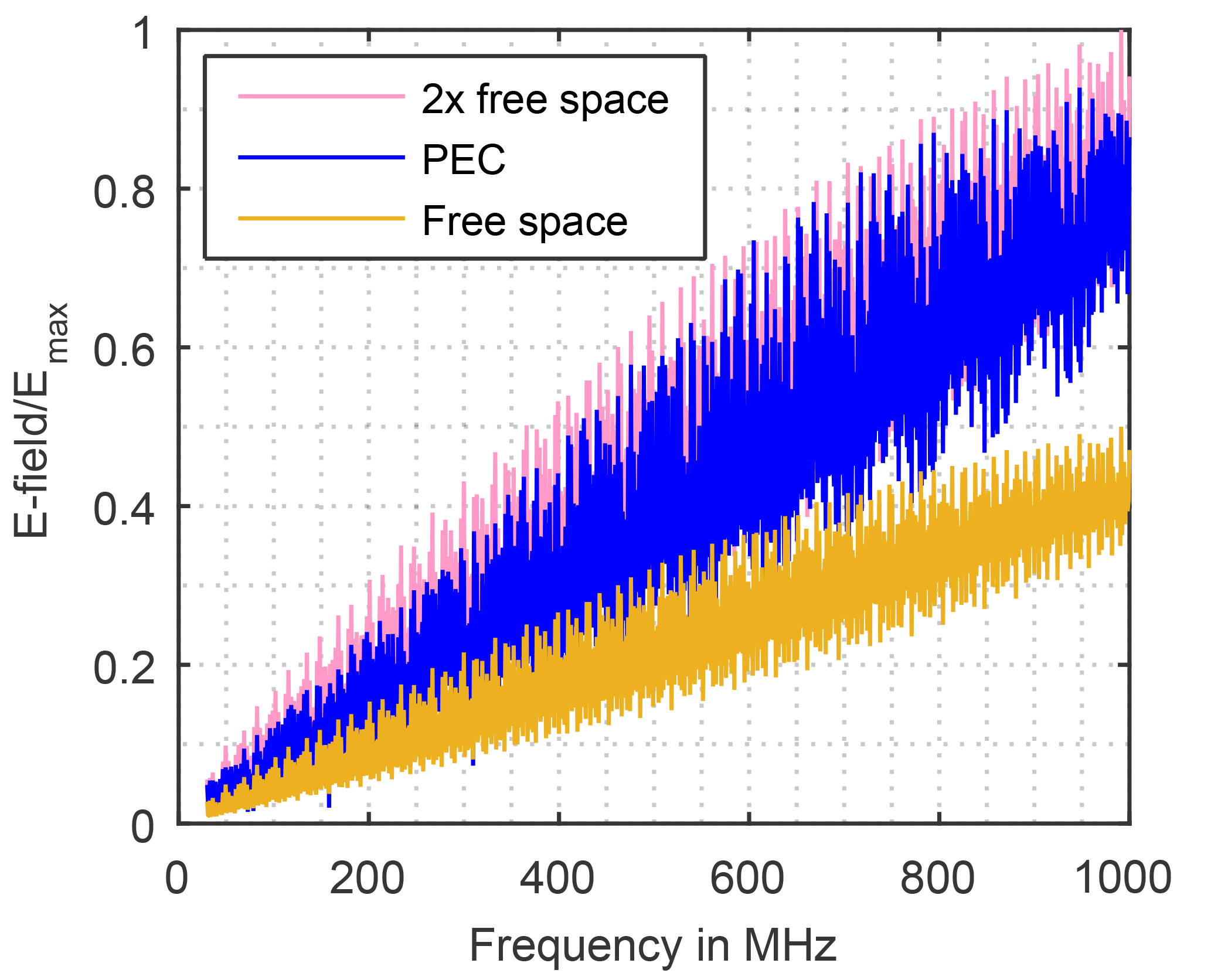
Figure 12 Validation of the simulation model. Electric field strength calculated in free space and over PEC.

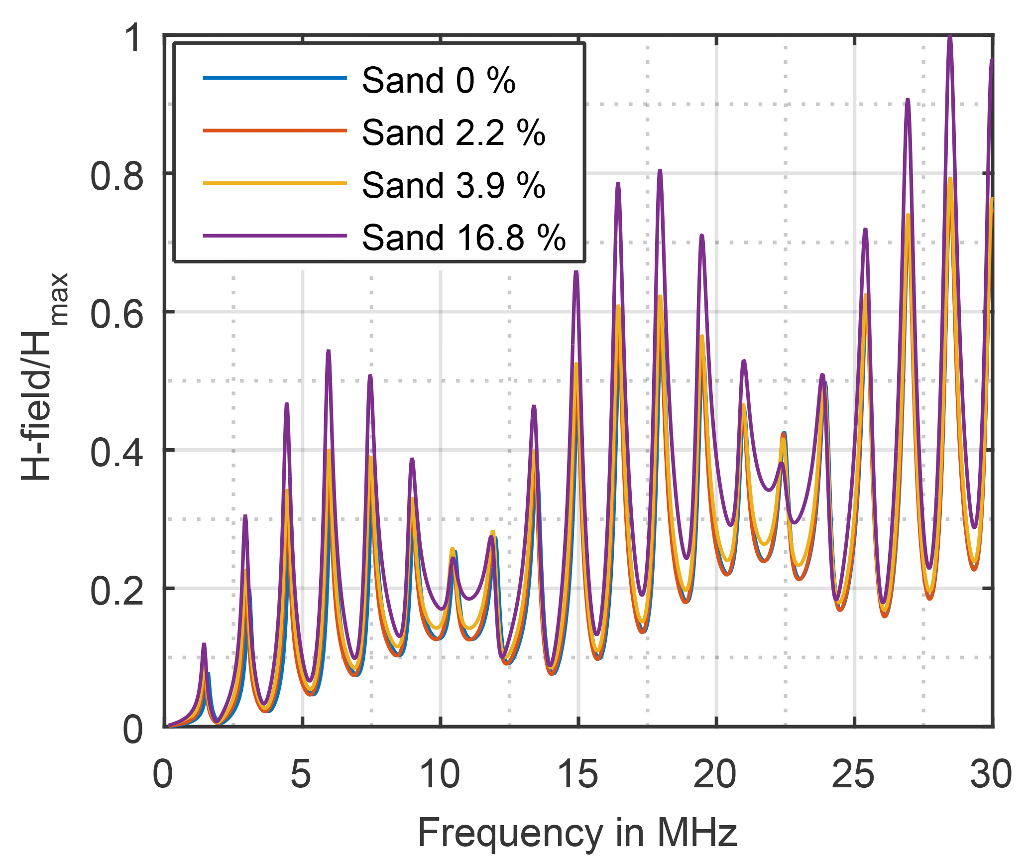
Figure 13 Magnetic field strength calculated over sand ground with various relative moisture rate.

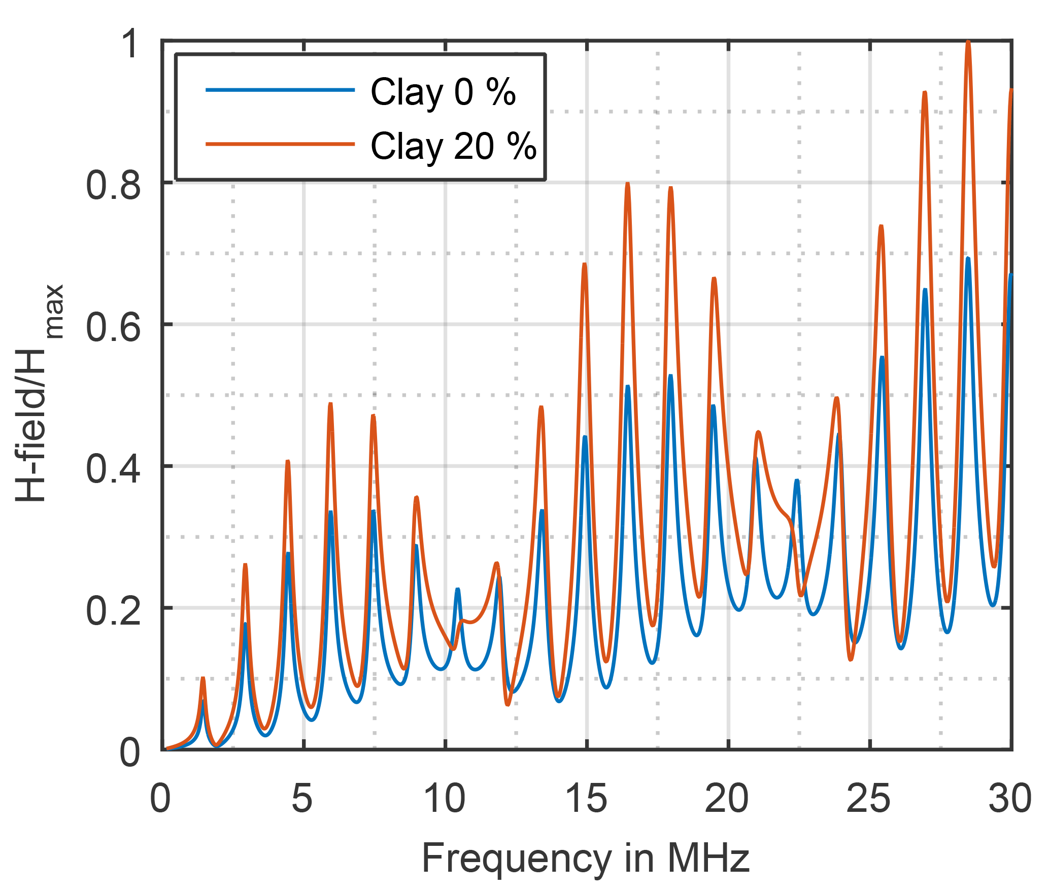
Figure 14 Magnetic field strength calculated over clay ground with various relative moisture rate.

In order to evaluate the impact on measurement uncertainty due to undefined ground the spectrum is divided into three parts based on the CISPR Bands B, C and D. Shown as an example, for the magnetic field with sand in Fig. 13 and with clay in Fig. 14 it is observed that the amplitude increases with increasing moisture rate, resonances occur proportional to the monopole`s length and the curve progression is similar for all moisture rates and both textures.

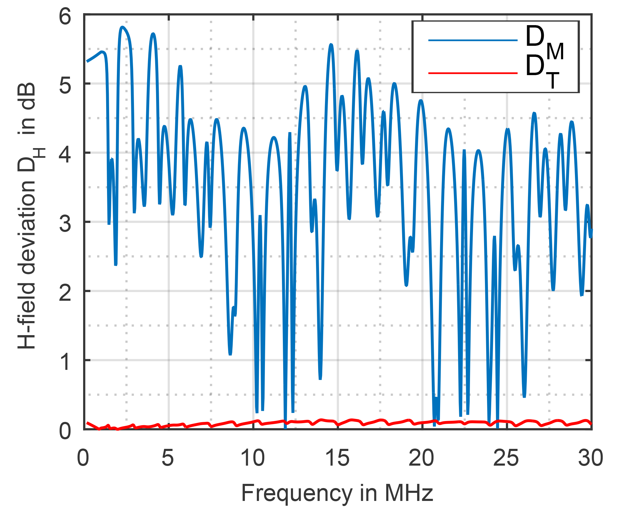
In order to differ between the texture's and the moisture rate's influence they are considered separately in the following. For the texture the deviation D_T is calculated by

$$\begin{array}{}\text{(11)}& D_{\mathrm{T}}=\mathrm{20}\left|\log \left({\displaystyle \frac{F_{\mathrm{S},\mathrm{0}}}{F_{\mathrm{C},\mathrm{0}}}}\right)\right|\end{array}$$

the field strength F_S,0 over sand as ground is dived by the field strength F_C,0 over clay as ground at zero moisture rate in each case. The deviation D_M of the moisture rate is calculated by Eq. (12), the field strength F_C,20 at maximum moisture rate (20.09 %, saturated ground) is divided by the field strength at zero moisture rate, of clay as ground.

$$\begin{array}{}\text{(12)}& D_{\mathrm{M}}=\mathrm{20}\left|\log \left({\displaystyle \frac{F_{\mathrm{C},\mathrm{20}}}{F_{\mathrm{C},\mathrm{0}}}}\right)\right|,\end{array}$$

While the deviation D_T due to different texture is low and has not to be regarded any further the deviation D_M due to different moisture rate is high, shown in Fig. 15 for the magnetic field and in Fig. 16 for the electric field.

Table 2 Standard measurement uncertainties caused by field reflection on undefined ground.

Figure 15 Deviation of the magnetic field strength.

Figure 16 Deviation of the electric field strength.

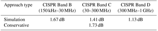
Supposing rectangular distribution, the uncertainty due to different moisture rate can be calculated by Eq. (13) taking each maximum deviation D_M, max occurring in the three frequency bands into account.

$$\begin{array}{}\text{(13)}& u_{\mathrm{M}}={\displaystyle \frac{D_{\mathrm{M},\max }}{\mathrm{2}\sqrt{\mathrm{3}}}}\end{array}$$

The results for the magnetic field strength (CISPR Band B) and the electric field strength divided in CISPR C and D Band are shown in Table 2.

6.2 Validation with a Conservative Approach

As shown in Sect. 6.1, the relative moisture rate is a significant factor for the measurement uncertainty. In consideration of extreme EM properties, ground with the relative humidity of zero percent, is assumed EM neutral behaviour, i.e. the WT is in free space. The field strength detected at this state corresponds to the value F₁ in Fig. 17. Taking into account the other extreme, ground is very wet or even seawater (offshore WT), i.e. the WT is on PEC. The field strength detected at this state corresponds to the value F₂ in Fig. 17. It is assumed that the field strengths F₁ and F₂ are detected at the same observation point and that the EM emissions of the WT remain the same for both scenarios. According to the law of reflection, the field strength F₂ can be considered a superposition of a direct field component and a indirect field component reflected at the PEC plane. Of interest in this consideration is only the constructive overlay, leading to a field increase and in worst case exceed the limits. In the scenario sketched, the field strength F₂ can be at twice as large as the field strength F₁, leading to a deviation of 6 dB. Assuming a rectangular distribution, this approach leads to a standard uncertainty of 1.73 dB.

Figure 17 Field strength PDF according to the conservative approach.

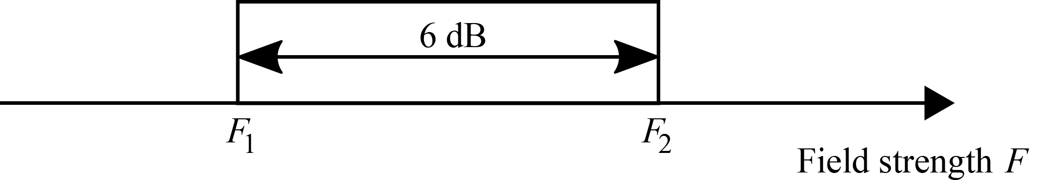
Table 2 summarizes the values of the standard measurement uncertainties due to undefined ground, derived in this work. It can be seen that the numerically obtained standard uncertainties are always smaller than the conservative uncertainty, validating the simulation results. However, it should be noted that the simulation results are only applicable to onshore WECS, but the conservative standard uncertainty is a general valid assumption, hence applicable to both, onshore and offshore installations.

7 Conclusions

The electromagnetic (EM) emissions of wind energy conversion systems (WECS) are evaluated in situ. Results of in situ tests, however, are only valid for the examined equipment under test (EUT) and cannot be applied to series production as samples, as the measurement uncertainty for in situ environments is not characterized. Currently measurements must be performed on each WECS separately, that is associated with significant costs and time requirement to complete.

Therefore, this work, explains the measurement of EM emissions of WECS. Evaluating the normative situation on the determination of EM emissions of WECS results in the definition of the magnetic (CISPR Band B) and the electric field strength (CISPR Bands C and D) as measurand.

In order to evaluate the measurement uncertainty, the measurands are described using model equations, based on the standard procedure according to the “Guide to the expression of uncertainty” (GUM). To determine the expected value and the associated measurement uncertainty of the measurand, knowledge of the so-called input values of the model equation is necessary.

Evaluation of the normative situation on measurement uncertainty of EM emission measurements leads to the result that open area test site (OATS) is the most similar test-site to in situ environment. Model equations for the measured field strength and input values specified for OATS can be adopted. Taking a closer look on the input values, two aspects occur with the need to further evaluation: the deflection of the antenna caused by wind velocity, and the reflection of EM fields on undefined ground.

In order to evaluate the deflection of the antenna tripod, caused by wind velocity, common antennas are simulated under different tilting angles in a plain wave field. The antenna foot point voltage, which directly relates to the EM field, is observed. By calculating the force necessary to tilt a common antenna tripod up to a certain angle and using the analytical characteristic of a dipole, the relation between wind velocity and deviation of the EM field is established. The EM field of tilted and not tilted antenna is compared and the impact on the standard measurement uncertainty is presented.

The reflection of the EM waves on undefined grounds is evaluated in two approaches. In the first one, a simplyfied model of a WECS is simulated above infinite extended ground with different EM characteristics. The observed EM fields of the extremes in texture and moisture are compared. This shows that the influence of varying ground moisture has a much higher influence on the measurement uncertainty than the variation of the texture.

Therefore, a second, conservative approach assessing the measurement uncertainty is derived from the law of radiation, taking the relative soil moisture into account. In summary, it can be said that the numerically obtained standard uncertainties are always smaller than the conservative uncertainty, validating the simulation results. However, it should be noted that the simulation results are only applicable to onshore WECS, but the conservative standard uncertainty is a general valid assumption, hence applicable to both, onshore and offshore installations. Thanks to the achievements made in this contribution it is possible to determine the measurement uncertainty of radiated EM emissions during WECS evaluation.