 | 19 Sep 2019
Measurement uncertainty caused by distance errors during in situ tests of wind turbines
Cornelia Reschka
Sebastian Koj
Sven Fisahn
Heyno Garbe
During the assessment of the electromagnetic emissions of wind turbines (WTs), the aspects of measurement uncertainty must be taken into account. Therefore, this work focuses on the measurement uncertainty which arises through distance errors of the measuring positions around a WT.
The measurement distance given by the corresponding standard is 30 m with respect to the WT tower. However, this determined distance will always differ e.g. due to unevenness of the surrounding ground, leading to measurement uncertainties. These uncertainties can be estimated with the knowledge of the electromagnetic field distribution. It is assumed in standard measurements, that the electromagnetic field present is a pure transversal electromagnetic field (far field). Simulations of a simplified WT model with a hub height of 100 m shows that this assumption is not effective for the whole frequency range from 150 kHz to 1 GHz. For frequencies below 3 MHz the field distribution is monotonically decreasing with the distance from the WT since it behaves like an electrical small radiator. Whereas for frequencies above 3 MHz, where the investigated model forms an electrical large radiator, the field distribution becomes more complex and the measurement uncertainty of the field strength at the observation point increases. Therefore, this work focuses on investigations where the near field becomes a far field. Based on the simulation results, a method for minimizing the uncertainty contribution caused by distance errors is presented. Therefore, advanced measurement uncertainty during in situ test of WTs can be reduced.
- Article
(4367 KB) - Full-text XML
- BibTeX
- EndNote


Every electrical system emits electromagnetic fields. Since these fields could disturb or harm other electrical systems, given limits have to be met. In the case of wind turbines (WTs), these limits are defined in the CISPR 11 (CISPR 11, 2015). For reproducible measurement results, not only are the limits defined, but also the measurement positions and frequency ranges. These definitions are further specified in a technical guideline (FGW/TR 9, 2016). For the measurement a minimum of 4 measuring positions at a distance of r30=30 m to the tower of the WT as shown in Fig. 1 are required. The magnetic field strength has to be measured in the CISPR Band B from 150 kHz to 30 MHz by using a loop antenna, the electric field strength shall be measured in the CISPR Bands C and D from 30 MHz to 1 GHz with a logarithmic periodic dipole antenna (LPDA) or a biconical antenna. A detailed description can be found in CISPR 11 (2015), FGW/TR 9 (2016) and Koj et al. (2018). However, without the knowledge of the measurement uncertainty, a serial release of WTs is not possible and therefore, the assessment of a WT is very time consuming and expensive.
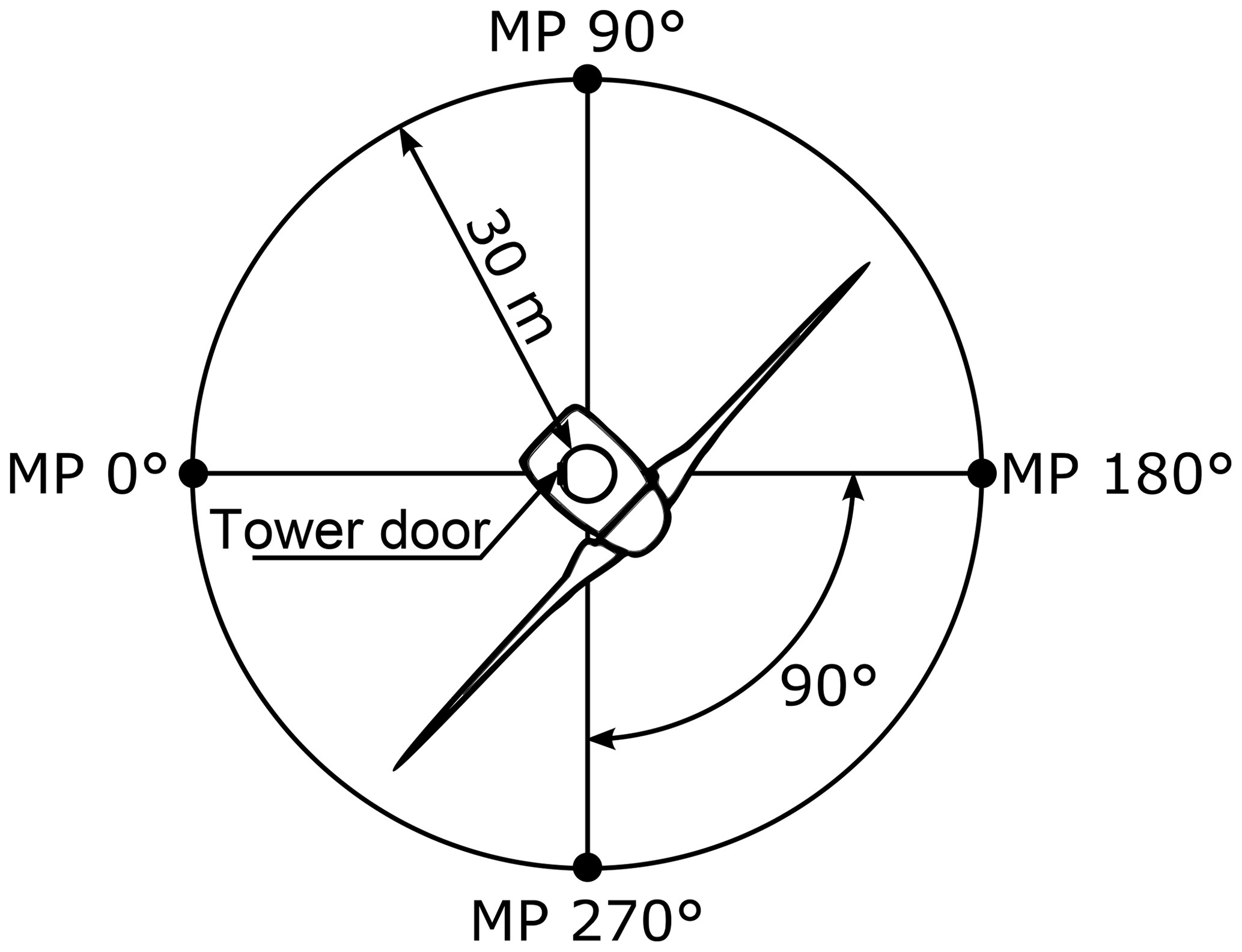
Figure 1Measuring positions according to FGW/TR 9 (2016).
When measuring the electromagnetic fields, one has to keep in mind, that every measuring result is afflicted by an expanded uncertainty. Therefore, the standard uncertainty has to be determined according to the “Guide to the Expression of Uncertainty” (GUM, 2008). To calculate the standard uncertainty, information about the uncertainty contributions are needed which had to be characterised for the in situ measurement. In previous works the contribution to the measurement uncertainty of the wind and of the undefined ground had already been investigated (Koj et al., 2018). In this contribution the influence of the uncertainty of the distance is presented.
Since WTs are tested in situ, there are various causes for the uncertainty of the distance. WTs are most often located in areas used for agriculture, the ground around the WT is uneven. This leads to an inaccurate placement of the antenna due to unsuitable ground at the determined measuring position or because of inaccuracies while measuring the distance to the WT due to the given circumstances. Furthermore, the measuring equipment itself can be the cause of some inaccuracies, e.g. the antenna phase centre of a logarithmic periodic antenna that is wandering with respect to the frequency. All these factors add up to the measurement uncertainty. This aspect is investigated in this work.
Therefore, in Sect. 2 the limits for the far field are considered for electrical small and for electrical large radiators. Following, in Sect. 3 the field distribution around a wind turbine is analysed based on simulation results in hindsight of the influence of the distance uncertainty to the WT. Thereafter, a method to minimize this uncertainty contribution is presented in Sect. 4. The conclusion in Sect. 5 gives a short summary of the most important insights of this contribution.
As mentioned before, the frequency range for the measurement stretches from 150 kHz to 1 GHz and has to be measured at a distance of r=30 m. To assess the electromagnetic emissions, the limits given in CISPR 11 (2015) are compared with the measured field strengths. To ensure the replicability of the measurement results, it is desirable to measure the field strengths in the so-called far field region. As commonly known, the far field only has transversal components, no longitudinal components, and the field impedance is the wave impedance of free space Ω. Various authors (Balanis, 2005; Kark, 2017; Gustrau, 2013) state that the far field of an Hertzian dipole starts at a distance of
Because of this, only frequencies above 20 MHz are assumed to be measured at the distance of 30 m in the far field. To investigate this assumption, a simulation model with an elementary electrical dipole was built with the help of the field solver FEKO from Altair Engineering GmbH (2015).
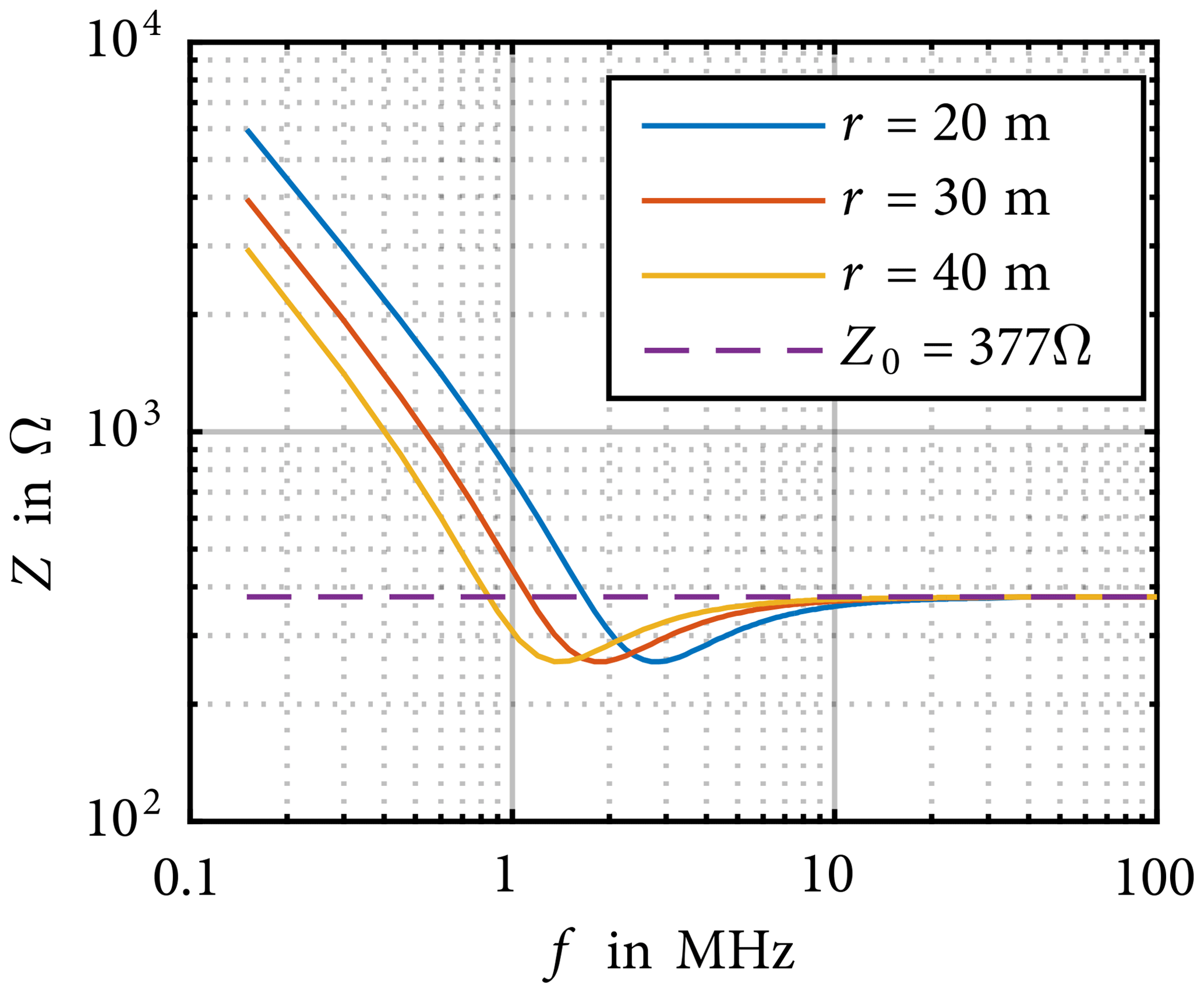
Figure 2Field impedance of a Hertzian dipole for different distances (Koj, 2019).
Figure 2 shows the calculated wave impedance for distances of 20, 30 and 40 m, as well as the wave impedance of free space Z0 over the frequency range from 150 kHz to 100 MHz. It is evident, that the field impedance gets closer to the free space wave impedance at about 2 MHz for 30 m distance and reaches the same values roughly in the range of 10 to 20 MHz. Since the wave length of 10 MHz is 30 m, the point of investigation is at a distance of one wavelength.
These results apply to electric elementary radiators and can also be used for small electric radiators. A radiator is electric small if the largest dimension Lmax of the radiator is less than the wavelength λ, according to Kark (2017)
Thus WTs with tower heights of hT≥100 m have to be regarded as electrical large radiators from about 3 MHz. For such, the far field distance can be assumed to be
according to Balanis (2005), Kark (2017).
With a tower height of hT=100 m and the maximum frequency of 1 GHz a distance of r=66.7 km would be needed. A measurement at this distance is not logistically possible, neither is a clear allocation of the measurement results to a certain WT possible. However, Laybros and Combes (2004) give the far field distance for the limiting case
with
which results in a distance of r=1200 m.
With these different definitions of the far field distance, a closer investigation for the case of a WT is done. Therefore, various distances are examined.

Table 1Investigated distances r between the WT model and the observation point.

In order to investigate which of those definitions best suits the WT, a simulation model is built to investigate four different distances. The model shown in Fig. 3 consists of a monopole with the length hT=100 m feed at the bottom via a voltage source. The whole model is placed over a perfect electrically conducted (PEC) ground plane. Using this model the electrical field E and the magnetic field H are calculated in varying distances r between the monopole and the observation point (OP). Whereby for CISPR Band B the OP is placed one meter above PEC and for CISPR Band C and D two meters above PEC. The investigated distances are listed in Table 1. With the calculated field strengths the wave impedance is obtained according to
In Fig. 4 the results are shown over the frequency range from 150 kHz to 30 MHz and in Fig. 5 from 30 MHz to 1 GHz. The coloured lines represent the different distances and additionally, the line for the distance of r=1200 m is dashed. For better comparison, all results are normalised to the free space wave impedance with
When the field impedance ZWT reaches the free space wave impedance Z0, the value will be zero. However, when the result of Eq. (7) is negative, it is a high impedance field and therefore the WT can be seen as an electrical field radiator. When the field impedance is positive, it is a low impedance field and therefore the source behaves as a magnetic field radiator. This recognition helps to identify the cause of the fields, i.e. the source of the interference. A high impedance field must therefore be caused by a voltage, a low impedance field by a current.
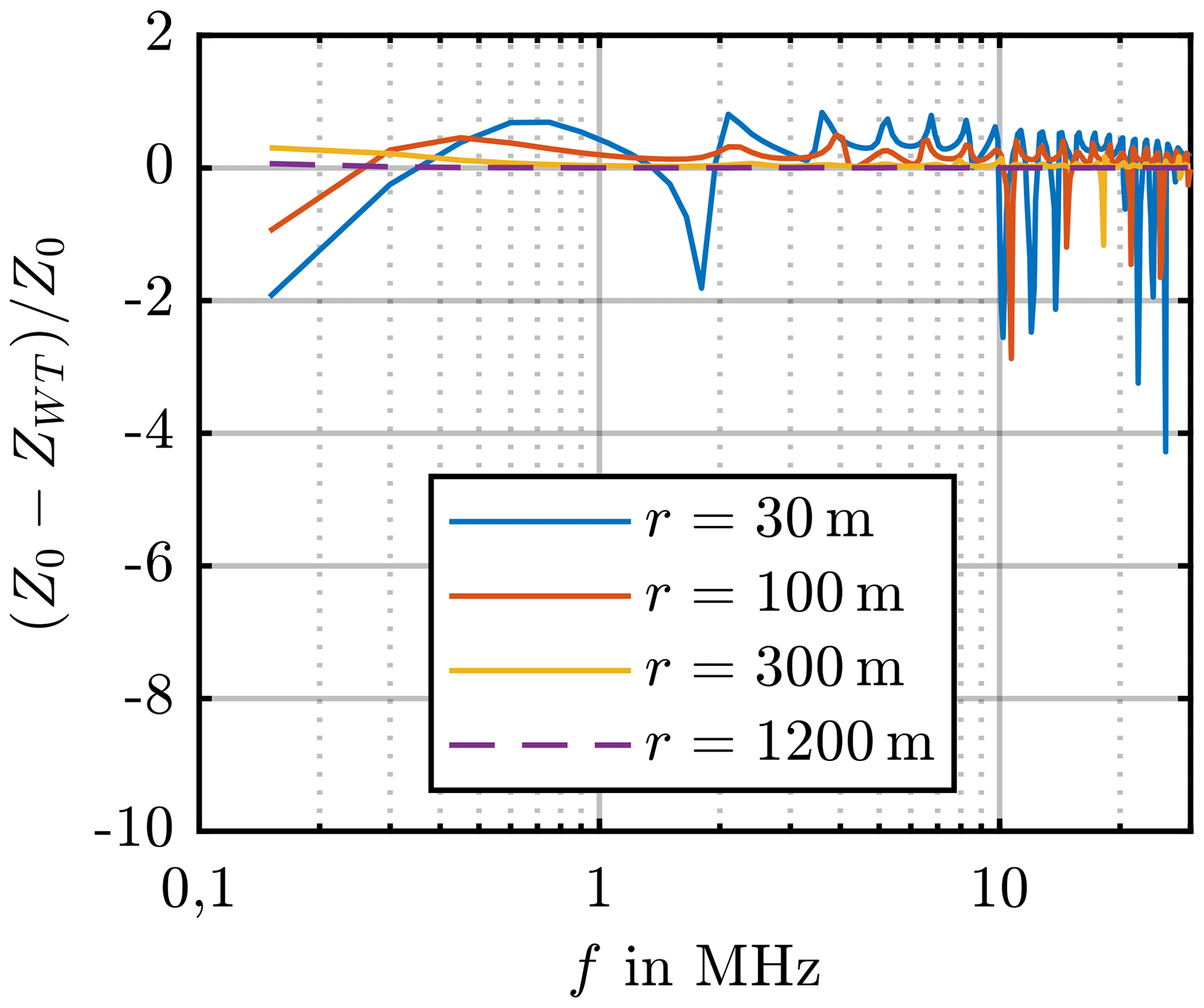
Figure 4Field impedance of a monopole over PEC for varying distances, frequency range from 150 kHz to 30 MHz.
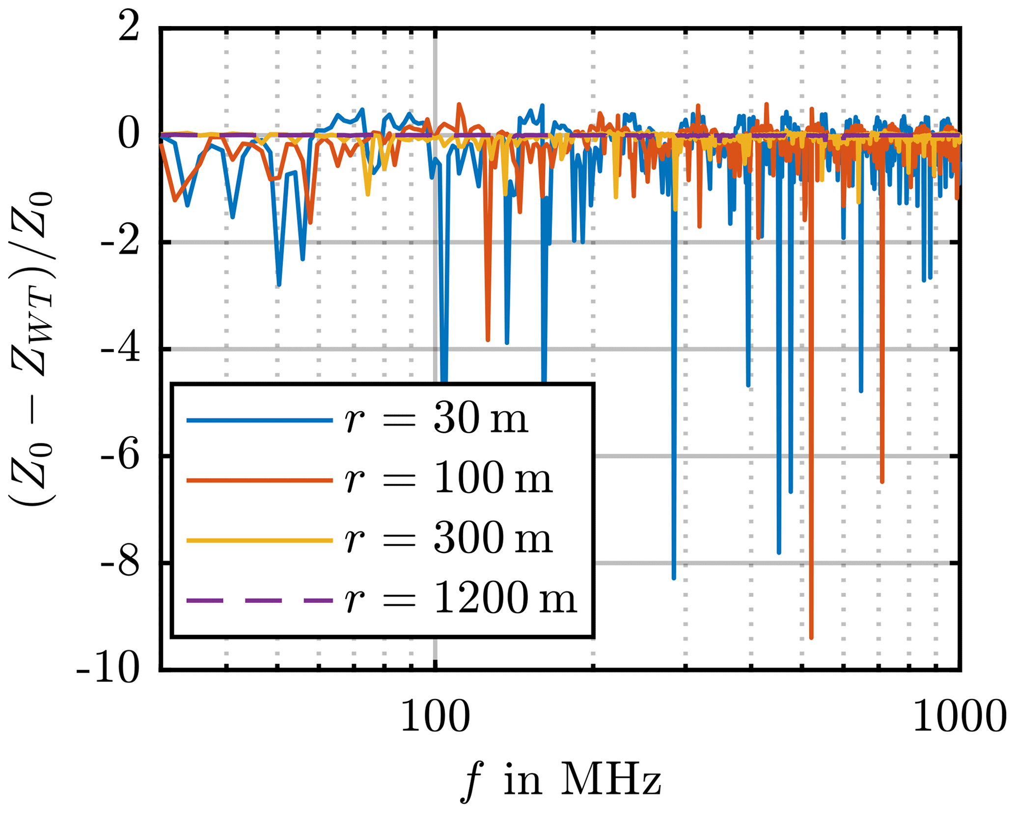
Figure 5Field impedance of a monopole over PEC for varying distances, frequency range from 30 MHz to 1 GHz.

Figure 6Magnetic field strength over the distance for discrete frequencies up to 3 MHz (Koj, 2019).
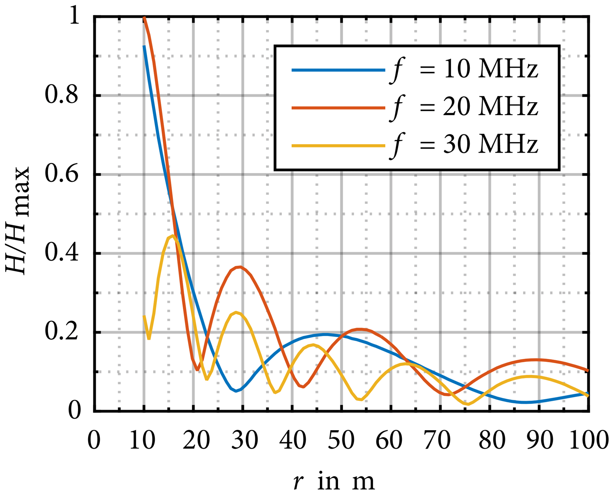
Figure 7Magnetic field strength over the distance for discrete frequencies above 3 MHz (Koj, 2019).
Figures 4 and 5 show that for the distance r=30 m given by the CISPR 11, the far field conditions for all three CISPR Bands cannot be reached. The orange line, which represents the distance r=100 m, shall reach the free space wave impedance at 3 MHz, but it is clear to see, that the line does not come close to zero, which means, that the free space wave impedance is not reached as expected. The yellow line, representing the distance r=300 m, shall reach the far field at 4.5 MHz. The line comes close to zero between 1 and 7 MHz, however, the field impedance shows greater differences to the free space wave impedance for higher frequencies. As mentioned previously, the distance r=1200 m is represented by the purple dashed line. It's clear to see, that for this distance the far field conditions are reached for the whole frequency range. This leads to the conclusion that a WT with a tower height hT=100 m can be examined in the far field at a distance of r=1200 m. The tower height has to be seen as the lower limit for electrical large radiators according to Eq. (5) and therefore the far field distance of a WT can be given with
In summary, it can be said that the measurements of the magnetic and electric field strength taking place at the normative required distance r30=30 m, are not in the far field at all required frequencies. Therefore, the need for the knowledge of the field distribution around the measuring position arises.
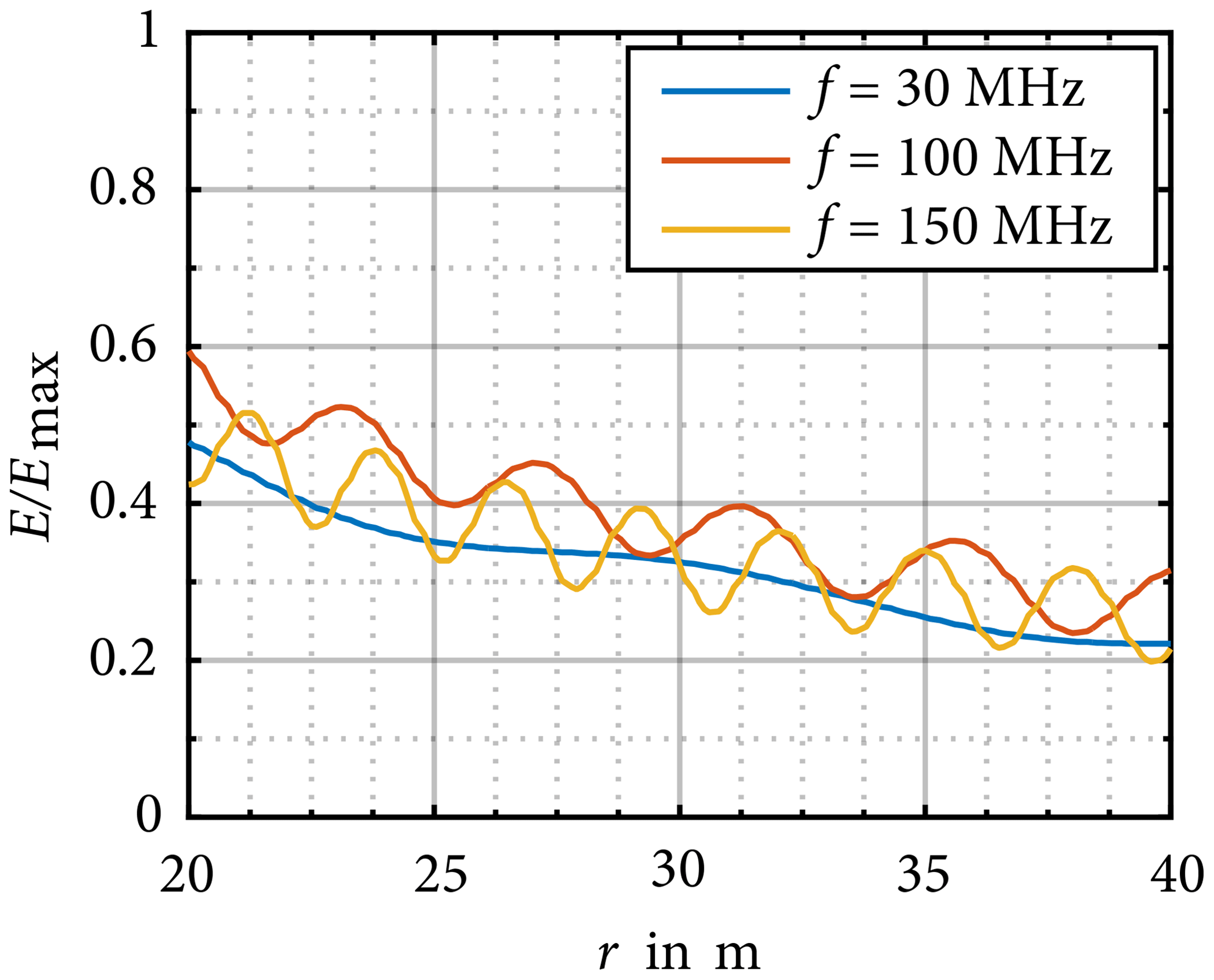
Figure 8Electric field strength over the distance for discrete frequencies up to 150 MHz (Koj, 2019).

Figure 9Electric field strength over the distance for discrete frequencies above 150 MHz (Koj, 2019).
In order to determine the uncertainty contribution of the distance error as described previously, the field distribution around a WT is investigated by the model shown in Fig. 3. In contrast to the previous simulations, now discrete frequencies are investigated over a varying distance r. The distributions of the magnetic field are shown in Figs. 6 and 7 for the distance . The results are normalized to the maximal magnetic field strength Hmax. Figure 6 shows the field distribution at the frequencies 150 kHz, 1 MHz, 1.5 MHz and 3 MHz. It can be seen that the field strength is decreasing monotonically for frequencies below 3 MHz, thus the model is an electrical small radiator. The simulation results for the frequencies 10, 20 and 30 MHz are shown in Fig. 7. At those frequencies the model has to be seen as electrical large and the field distribution is not decreasing monotonically. Furthermore, the phenomena of standing waves can be observed due to reflections on the PEC ground.
In order to investigate the distribution of the electric field strength, simulations for distances are calculated. The results are shown in Figs. 8 and 9 for different frequencies between 30 MHz and 1 GHz, whereby the results of the electric field strength are normalised to its maximum Emax. In this frequency range the WT also behaves like an electrical large radiator and standing waves occur in the electric field distribution similar to Fig. 7. The standing wave can be characterised by its local minima and maxima. The distance between the maxima decreases with increasing frequency.
With the knowledge of the field distribution, the influence of the distance error on the measurement uncertainty of the field strength can be explained. For example, the electric field strength distribution at 300 MHz in Fig. 9 shows a local maximum at the distance r30=30 m. In the case of the antenna being located with a distance error Δr near r30, a different field value will be measured.
If a logarithmic periodic dipole antenna (LPDA) is used for the measurement of the electric field strength, a distance error of m caused by wandering phase centre along LPDA can be assumed. Finally, the resulting field uncertainty ΔF caused by Δr can be written as
Using Eq. (9) and the simulated field distributions, the resulting field uncertainty can be calculated for each frequency range, as shown in Figs. 10 and 11. Figure 10 shows, that in the frequency range below 10 MHz, the expected uncertainty does not exceed ±1 dB. However, for higher frequencies uncertainty values of up to ±6 dB are possible as seen in Fig. 11.
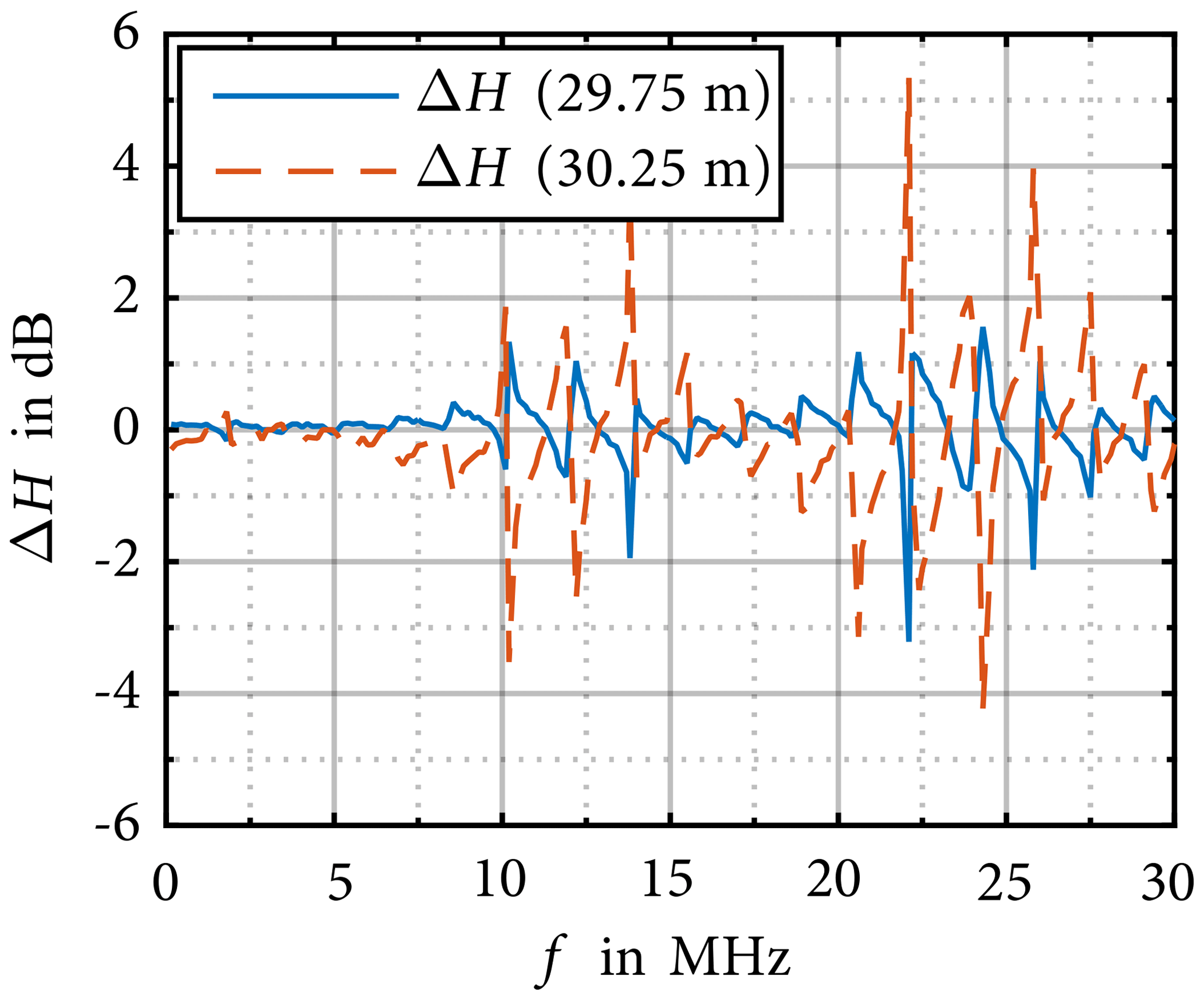
Figure 10Uncertainty contribution caused by distance errors for the magnetic field strength (Koj, 2019).
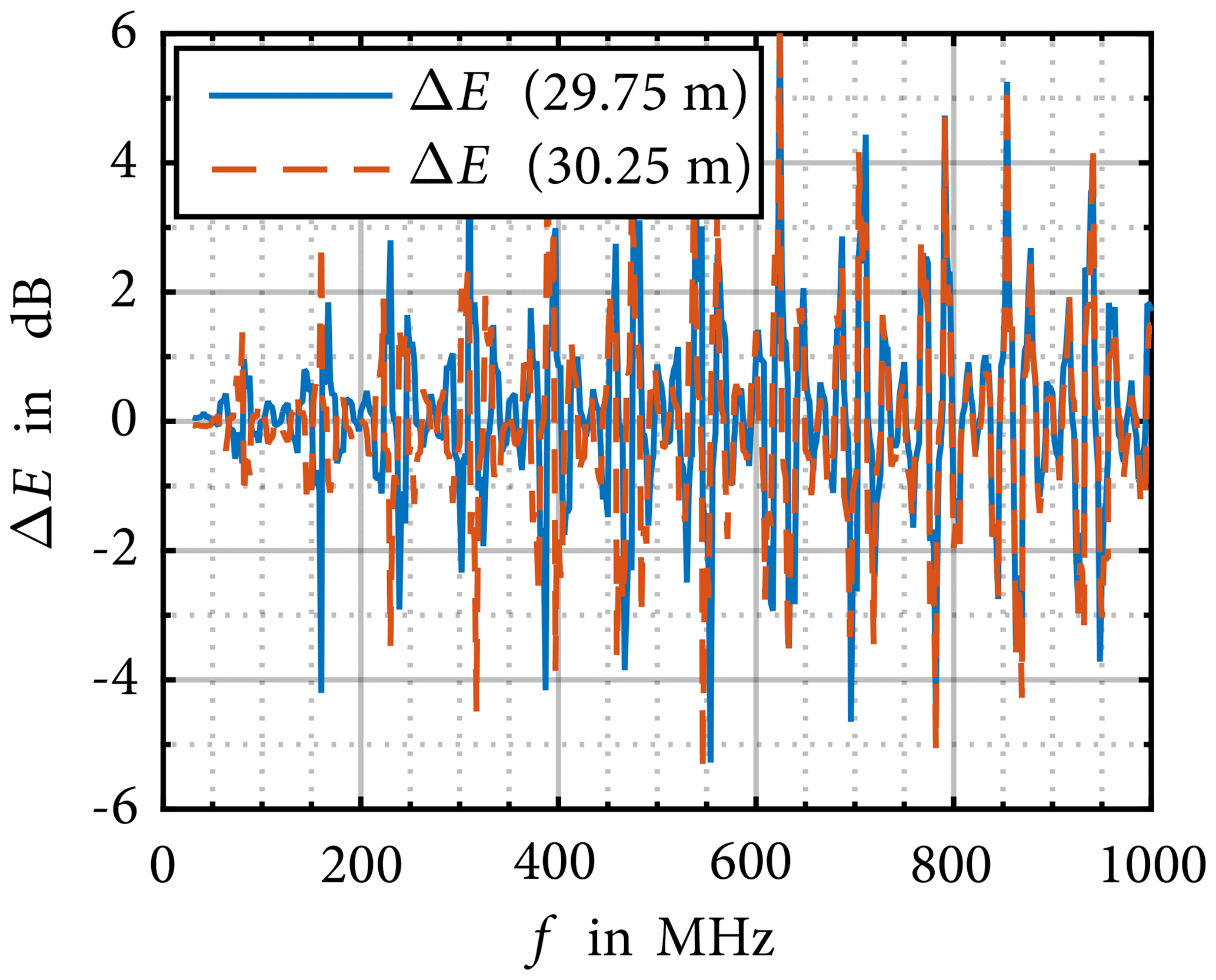
Figure 11Uncertainty contribution caused by distance errors for the electric field strength (Koj, 2019).
Since the wavelength decreases with increasing frequency, the error made becomes greater with increasing frequency. Therefore, a way to minimize the uncertainty contribution caused by distance error is needed and is treated in the following section.
The goal of this chapter is to define a method which allows a reduction of the measurement uncertainty described above, the influence of the frequency and of the tower height hT on the field distribution is investigated. Figures 7, 8 and 9 show that the distance between two maxima of each field distribution decreases with increasing frequency. Figure 12 shows the magnetic field distribution at 30 MHz for different tower heights. It can be seen that the location of each local maxima depends on the tower height. Furthermore, it is seen that the local maxima of the field distribution decreases with the distance r according to 1∕r.
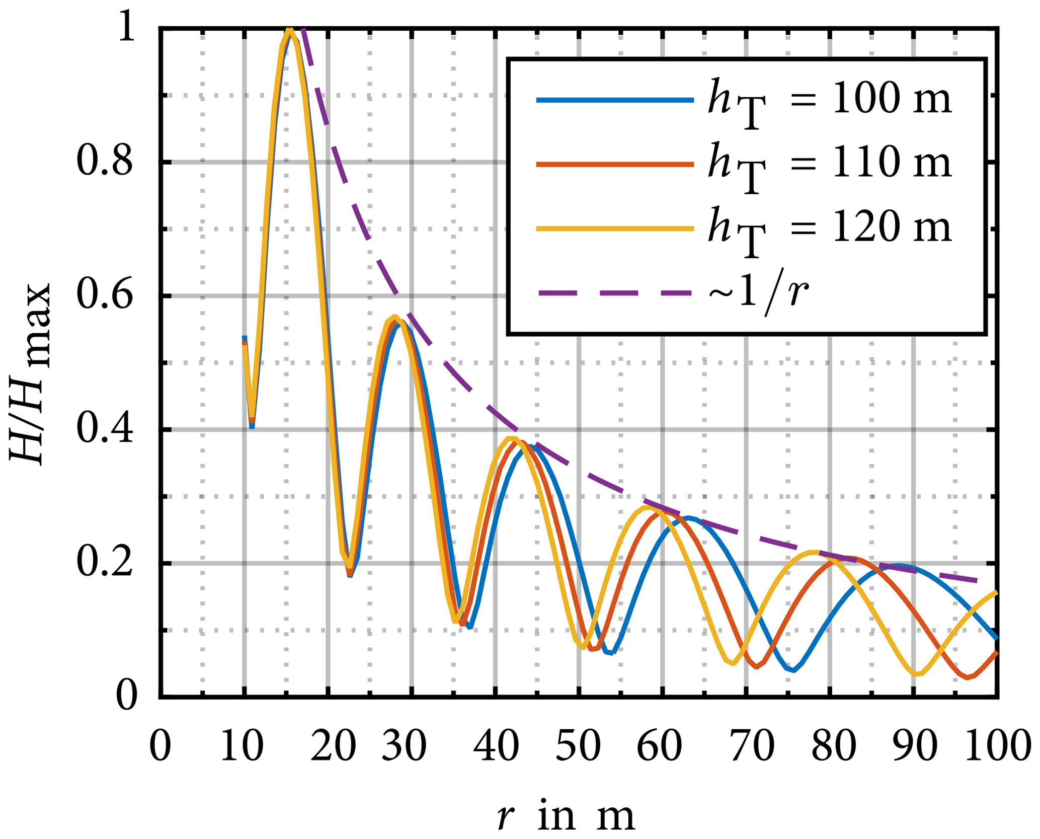
Figure 12Field distribution for different tower heights at 30 MHz (Koj, 2019).
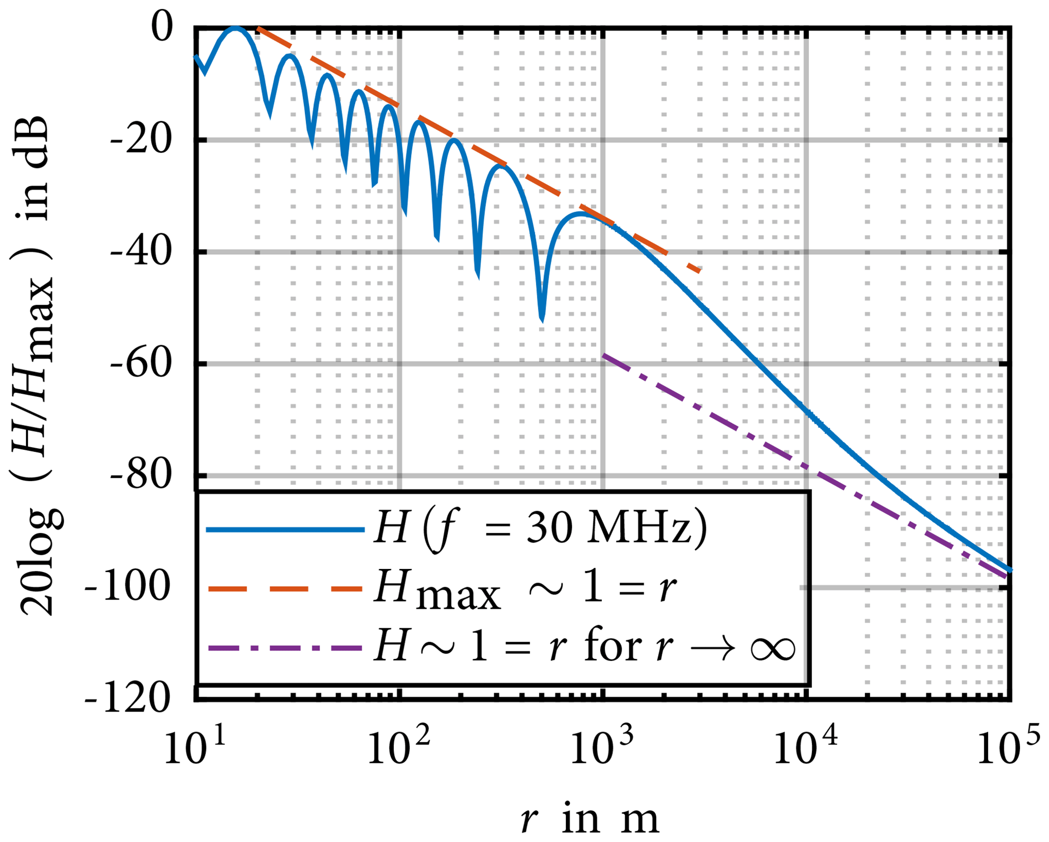
Figure 13Field distribution for 30 MHz at a tower height hT=100 m (Koj, 2019).
Figure 13 shows the magnetic field distribution at 30 MHz for a WT model with hT=100 m for distances of . For a better presentation, the distance r is given logarithmically. It can be seen, that the local maxima occur till r≈1 km and decrease with 1∕r. For distances r>1 km the field distribution is falling monotonically and follows 1∕r for distances above 10 km. Far field conditions can be expected at those distances.
The idea of reducing the influence of the distance errors and the measurement uncertainty of the magnetic and electric field strength is based on the 1∕r dependence of the local maxima of each field distribution. Therefore, the field distribution should be scanned near the measuring position r30 along the distance r to ensure that the maximum field strength Fmax is measured. Here, the distance between the WT tower and the position of the local field maximum rLM has to be determined as well. Using both the measured maximum field strength Fmax and the corresponding distance rLM, the field strength F30 at the normative required distance r30=30 m can be calculated using 1∕r dependence of the field distribution
Finally, the calculated field strength can be compared with the given limits.
This work describes the contribution of distance errors to the measurement uncertainty during in situ tests of electromagnetic emissions of wind turbines (WTs). In order to investigate the far field region, a simple model of a WT is set up and numerically analysed. The simulation results show that at the normative required distance of r=30 m and in the frequency range from 150 kHz to 1 GHz far field conditions cannot be expected.
Therefore, the field distribution near a WT is calculated. It can be shown that at those frequencies, where the WT model is an electrical small radiator, the field distribution shows a monotonically decreasing dependence on the distance r. For this case, the resulting measurement uncertainty of the field strength is smaller than ±1 dB. For those frequencies, at which the WT behaves like an electrical large radiator, the resulting field distribution can be described with standing waves, i.e. local minima and maxima occur. For this case, the resulting measurement uncertainty increases.
In order to reduce the measurement uncertainty at electrical large radiators, the dependence of the field distribution from the frequency and the tower height is investigated. It is shown that the distance between two maxima of the field distribution decreases with increasing frequency. The location of a local maximum also depends on the tower height. However, the simulation results show that the levels of the local maxima decrease with distance r according to 1∕r. Using this fact, a simple method to reduce the measurement uncertainty is given. For this purpose, the field strength has to be scanned near the measuring position along the distance r till a local maximum is found. Finally, the measured maximum field strength must be calculated for the given normative measuring distance.
Using the presented results, the measurement uncertainty of in situ tests of radiated electromagnetic emissions from WTs can be described. With the knowledge of this uncertainty a serial release of WTs is possible. The assessment of WTs becomes more time and cost effective.
The data are available from the corresponding author upon request.
All authors contributed to the design and implementation of the research, the analysis of the results and the writing of the manuscript.
The authors declare that they have no conflict of interest.
This article is part of the special issue “Kleinheubacher Berichte 2018”. It is a result of the Kleinheubacher Tagung 2018, Miltenberg, Germany, 24–26 September 2018.
The publication of this article was funded by the open-access fund of Leibniz Universität Hannover.
This paper was edited by Thorsten Schrader and reviewed by two anonymous referees.
Altair Engineering GmbH: Altair FEKO, Calwer Straße 7, 71034 Böblingen, Germany, available at: http://www.feko.info, http://www.altair.com (last access: 8 July 2019), 2015.
Balanis, C. A.: Antenna Theory, 3rd Edition, John Wiley & Sons, New Jersey, USA, 2005.
CISPR 11: Industrial, scientific and medical equipment – Radiofrequency disturbance characteristics, Limits and methods of measurement, International Electrotechnical Commission, 2015.
FGW/TR 9: Technical Guidelines for Wind Turbines (FGW Guideline) Part 9:2016, Rev. 1, Determination of High Frequency Emissions from Renewable Power Generating Units, FGW e.V. – Fördergesellschaft Windenergie und andere Dezentrale Energien, 2016.
GUM: JCGM 100: Evaluation of measurement data, Guide to the expression of uncertainty in measurement, 2008.
Gustrau, F.: Hochfrequenztechnik: Grundlagen der mobilen Kommunikationstechnik, 2nd edn., Fachbuchverlag Leipzig, München, Germany, 2013.
Kark, K. W.: Antennen und Strahlungsfelder, 6th Edition, Springer Vieweg, Wiesbaden, Germany, 2017.
Koj, S.: Messunsicherheit bei in situ Tests der elektromagnetischen Verträglichkeit von Windkraftanlagen, sierke Verlag, Göttingen, Germany, 2019.
Koj, S., Hoffmann, A., and Garbe, H.: Measurement Uncertainty of Radiated Electromagnetic Emissions in In Situ Tests of Wind Energy Conversion Systems, Adv. Radio Sci., 16, 13–22, https://doi.org/10.5194/ars-16-13-2018, 2018.
Laybros, S. and Combes, P.F.: On Radiating-Zone Boundaries of Short, λ∕2 and λ Dipoles, IEEE Antenn. Propag. M., 46, 53–64, 2004.
- Abstract
- Introduction and motivation
- Consideration of the far field region
- Field distribution around a wind turbine and uncertainty contribution
- Method to minimize the uncertainty contribution
- Conclusion
- Data availability
- Author contributions
- Competing interests
- Special issue statement
- Financial support
- Review statement
- References