Estimation of ionospheric reflection height using long wave propagation

Phase height measurements of low frequency radio waves are used to study the long-term variability of the mesosphere over Europe. Phase height measurements use a characteristic pattern in field strength registration of radio waves interpreted as phase relations between sky wave and surface wave to obtain the apparent height of the reflection point, the Standard Phase Height (SPH). Based on this SPH-method a homogenized daily series was generated since 1959 at Kühlungsborn. Improvements of the measuring method show that the signal is significantly influenced by lower atmospheric layers. Mesospheric reflection is not the exclusive source of the measured behavior. Tropospheric influence can not be neglected. Taking this into account one has to conclude that the strong coherency of the SPH data to mesospheric heights is not as significant as previously assumed.

1 Introduction

Indirect phase height measurements of long wave radio frequencies are a common method in order to study the long-term variability of the D region in the ionosphere. Field strength measurements have been maintained since February 1959, after the International Geophysical Year 1957/58, in Kühlungsborn (e.g., Entzian, 1967; Bremer and Peters, 2008). The results can be used as an indicator for climate changes, which are nowadays important for the society (Peters and Entzian, 2015). Peters found a decrease of 114 m per decade in SPH. It is based onto the assumption that the field strength variations known as Hollingworth pattern (Hollingworth, 1926) is only caused by a change in mesospheric reflection height. Refinements and additional measurements suggest that the observed Hollingworth pattern are also influenced by lower atmospheric layers. It is possible that the influence of the lower layers is even much greater than previously assumed (Bracewell et al., 1951; Entzian, 1967, 1972; Lauter et al., 1984; Taubenheim et al., 1997). The focus in this article is laid to clear some inconsistencies related to the measuring path from Allouis (47^∘ N, 2^∘ E, Central France) as broadcasting station to Kühlungsborn (54^∘ N, 12^∘ E, Northern Germany), which is located about 1023 km away and serves as receiving location.

2 Model, analysis method

The diurnal amplitude pattern (upper panel a) in Fig. 2 of an VLF radio station is usually interpreted as a superposition of the ground wave following the Earth's surface and the sky part reflected at ionospheric layers. Figure 1 shows the geometry which is supposed in our case. For a phase difference between the waves of n⋅λ (with λ as wave length and n as an integer) a maximum is observed, and for a difference of $\mathrm{0.5}+n\cdot \mathit{\lambda }$ a minimum. This approach allows to compute corresponding apparent heights h (panel b) in Fig. 2, although the ambiguity has to be solved. Introducing the Chapman function as x-axis one can find a linear relation between h and ln (Chap(χ)) (χ being solar zenith angle) on a daily basis (Lauter, 1984). The slope H and a zero height h₀ are obtained by linear regression using the observed times of occurrence of the extremes and the corresponding heights. A zenith angle that appears during all seasons at the radio link path is χ=78.4^∘ (cos (χ)=0.2). This zenith angle is used to find a daily height value SPH via H and h₀ (Fig. 3). This way one get a time series with one value daily, which is slightly removed from seasonal effects regarding the sun position.

Figure 1 Assumed geometry of wave paths.

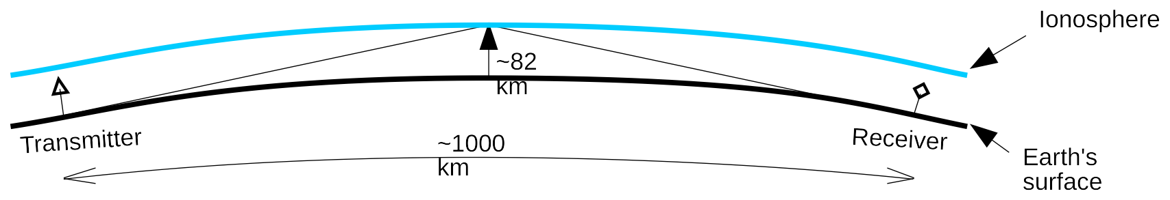
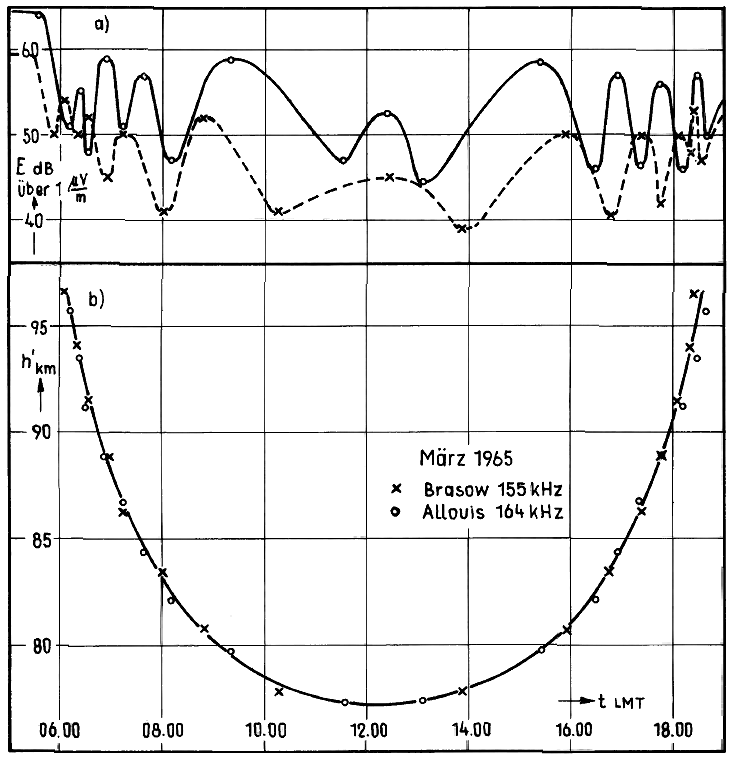
Figure 2 Hollingworth pattern (a), Relationship apparent height versus time (b) from Entzian (1967).

Considerable doubts in this simple geometric approach result from the analysis of the data around February 1986. At this time the frequency of the radio station used for the measurements was slightly lowered by 1.22 %. This implicates also changes in the evaluation formulas regarding the height scale. Furthermore one have to debate whether or not physical relationships changes due to the frequency shift. Through an estimation using electron density profiles the reflection height would decrease by less than 80 m, which can be neglected (Singer, 2013). This means the straight line in Fig. 3 should not change neither in the slope H nor in h₀. Hence, any jumps at the day of frequency change should not be visible neither in SPH nor in H and h₀ after applying the new height scale reflecting the new frequency. Figure 4 shows a comparison of data following the suggested corrections in the formulas or not. The visible jumps in the data, after applying the corrections, are shown in Fig. 4a, c. This indicates that the geophysical interpretation of the data has to be revised. It seems do be, that the underlying geometric model is wrong. This has a great influence on the interpretation of the SPH regarding long term issues. The decrease of 114 m per decade would be much greater because the data after 1986 are shifted upwards by 600 m due to the corrections.

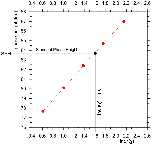
Figure 3 Linear relationship between apparent height and ln (Chap(χ)) with χ as solar zenith distance. Modified from Peters and Entzian (2015).

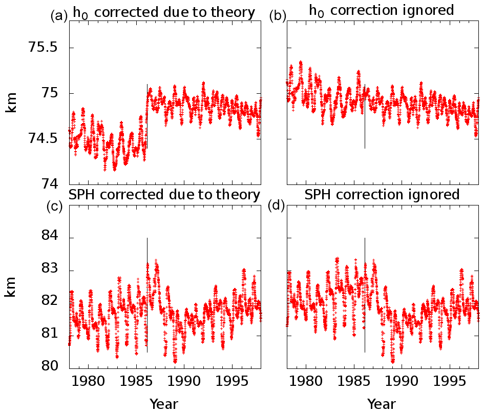
Figure 4 Comparison of data reflecting the model change due to frequency shift (a, c) or not (b, d). Panels (a) and (b) show h₀, panels (c) and (d) show SPH. Although the jump in SPH data is (c) not so easy to detect it is clearly visible in h₀ (a). The black lines indicates the date of the frequency shift.

3 Improvements in receiver technique

To get more resilient data, an additional measuring path Allouis–Juliusruh was set into operation in 2010. The distance is 100 km longer compared with the Allouis–Kühlungsborn path and the bearing is nearly the same (Juliusruh 54^∘ N, 13^∘ E, Northern Germany). Furthermore, both receivers were equipped with an GPS disciplined frequency normal. This opens the opportunity also to determine the absolute phase of the received signal with an accuracy of a few tens of nanoseconds. Expressed as phase angle φ, this is 3^∘. A shielded aperiodic loop coupled via a transformer was deployed as the antenna. After amplifying and low pass filtering of the signal it is directly delivered to an analog to digital converter. Frequency selection is done afterwards by FFT using computer technology. In this way, a measurement series with a time resolution of 5 s is obtained. The procedure to calculate the daily SPH value is not changed and carried out as described above. Both receivers are build up as a two channel version. Each channel is seeded by its own antenna which are entangled by 90^∘.

4 Results

4.1 Amplitude pattern

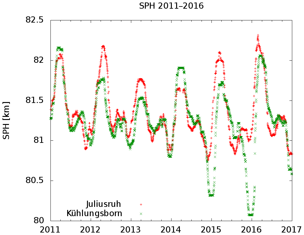
Subsequently are listed some effects that cannot easily be explained by the simple reflection model. Figure 5 shows the SPH for both measuring paths i.e. Allouis–Kühlungsborn and Allouis–Juliusruh for a few years. Noticeable are the differences in springtime which are roughly 400 m in height. Taking into account that the reflection point of both paths is only 50 km apart these differences seems to be much too large. One would expect a few 10th of meters. Since it is an apparent height and diffraction is neglected. The involved real reflection area is probably greater than 50 km in diameter. If this is not the case, a considerable inclination of reflecting layer must be assumed, which could be also a source for changes in field strength recorded at the receiver place. In this case one would record a value representing a tilting factor and not an apparent height.

Figure 5 SPH data deduced from reception in Kühlungsborn (green) and Juliusruh (red).

4.2 Antenna alignment

An other experiment was carried out using two antennas distorted by ±45^∘ against the bearing to the transmitter. The amplitude of both channels are decreasing by a factor of 0.707 due to cosine law, but they should be equal all the time. This is only the case a few hours around noon. But there are differences between both channels (Fig. 6). Just before sunset at 18:01 UTC one can find a minimum in one channel were in the other channel a maximum occurs. The reason for the differences could be for example a bending of the radio path or Faraday rotation effects. Research on extremely low frequencies (ELF) using wave guide theories (Mlynarczyk et al., 2017) shows a deviation of 10^∘ for the angle of arrival. This occurs if the day night border is within the propagation path due to different phase velocities for day and night. For the own measurements the amplitude differences in both channels depicted in Fig. 6 allow to assume a deviation angle of up to 20^∘. The occurrence of the differences around sunset reveal similarities to the ELF case. Ignoring this thoughts, and calculating the SPH for each channel individually one would result in a SPH height difference of about 2.5 km. This is quite large against the SPH decrease of 114 m per decade.

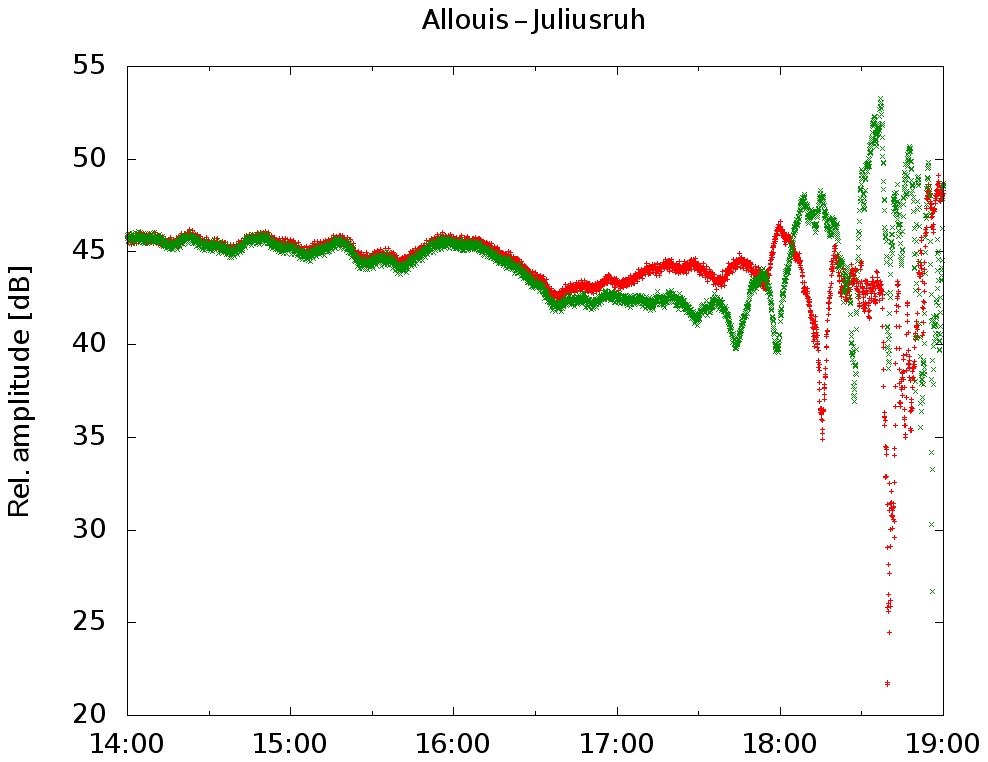
Figure 6 Example (7 September 2018) of recepion amplitude recorded in Juliusruh using two antennas distorted by ±45^∘. A calculation of SPH of each channel separately would give a height difference of about 2.5 km.

4.3 Direction finding

Following Fig. 1 and computing the elevation angle ε of the sky wave one obtains ε=6.6^∘. This low value makes it difficult to design an antenna which is able to distinguish between the incoming sky wave and the surface wave. A first approach to get elevation related values was to use a rotating ferrite rod in minimum bearing plane, which means that in the 90^∘ position the rod is horizontally aligned, while 0^∘ represents upright position. Figure 7 shows the result swinging the rod in 15^∘ steps. The 90^∘ sampling (light brown) shows the usual Hollingworth pattern known from the registration carried out since 1959 which has a loop antenna positioned in maximum bearing plane, but obviously with a much lower amplitude. Samples taken from an antenna orientation nearer to the upright position illustrate a completely different behavior. There might be a connection with gravity waves. The normal Hollingworth amplitude pattern is fading away while the antenna is approaching to its upright position. One would actually expect the opposite behavior. Conjecturally the incidence angle of the radio wave is far away from ε=6.6^∘.

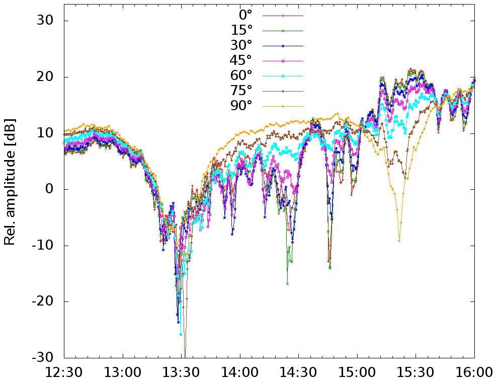
Figure 7 Reception amplitudes using a rotating ferrite rod. Indicated angles are taken against the upright position. The 90^∘ recording shows a behavior quite similar like the usual Holingworth pattern.

4.4 Phase and Amplitude

As the receiver is equipped with its own stable reference oscillator and furthermore the carrier of the used broadcast station at Allouis is seeded by a cesium fountain it is possible to record the absolute in-phase and quadrature component, known as complex amplitude or phasor. Figure 8a depicts a typical example of the amplitude recording over time, while the right part shows the coarse of the phasor. Each point in the plot is composed as addition of two vectors. A constant one which is representing the surface wave and a variable part depicting the sky wave. This is not so clear in the illustration on the right, because the phase has bin lost there. With time as parameter in the panel (b) the phasor starts in this plot at sunrise, rotating anticlockwise (red crosses). Usually two rounds can be observed each day under quiet sun conditions. From local noon on wards (green crosses) the rotating direction changes. Again after roughly two rounds the phasor ends here in the plot at sunset. The night time is not illustrated. Assuming a sky wave changing in amplitude and phase and a constant surface wave, then the addition of the two vectors should describe a spiral with a constant center. Obviously this is not the case in Fig. 8b. In order to explain the pattern one have to assume either that the surface wave is not constant or that there must be a third wave, unknown so far.

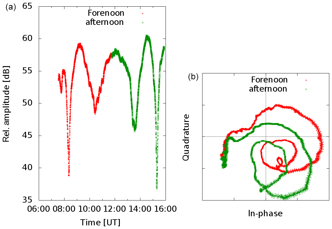
Figure 8 A typical example of the usual amplitude recording (a) Same data as the course of phasor with time as parameter, starting at sunrise, color change at local noon and ending at sunset (b).

4.5 Tropospheric effects

One remarkable occurrence could be observed on 5 May 2015. At this day a heavy tornado destroyed almost all houses in the town of Bützow (53^∘54^′ N, 11^∘59^′ E). It is a strong indicator for heavy local disturbances in lower atmospheric layers. The town is 29 km apart from Kühlungsborn and 2 km aside the pathway Allouis–Juliusruh. The Kühlungsborn recording shows no untypical pattern. But in Juliusruh the recordings are quite unusual (Fig. 9a). The oscillation period is about 6 min. Up to 10 circles always rotating clockwise can be detected in the phasor plot (Fig. 9b) during this event. Different colors are used to indicate the time for the rounds that are taken. The amount of rounds is 5 times greater as the usual daily movement of the phasor depicted in Fig. 8b. As this effect is only visible in the Juliusruh recordings and almost invisible in the Kühlungsborn data, it has to be a quite local effect. Furthermore, this is an unmistakable indication that the lower atmospheric layers must be taken into account for propagation measurements.

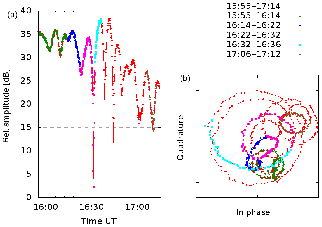
Figure 9 Amplitude (a) and Phasor (b) during heavy tropospheric disturbances. Colors indicate time periods for better overview.

4.6 Run time experiments

Summarizing the above mentioned experiments it seems impossible to gather separate information from the involved two wave components. Too many questions are still be open. Surely one would gain substantially more information with a pulsed system like a ionosonde. Oblique ionograms are available from Juliusruh since 2015. Unfortunately, they are starting only from 1.5 MHz, which is too far away from 162 kHz, which are the subject here. As the new receiver is a capable to receive the whole LF band the idea came up, to use the signals of the LORAN-C system. LORAN-C is a naval navigation system using LF pulses at 100 kHz. The technical parameters can be fond, for example, in Mills (1992), Pelgrum (2006) and U.S. Department of transportation (1994). The LORAN system was unfortunately decommissioned in December 2015, except for one transmission station at Anthorn (54^∘ N, 3^∘ W). The LORAN pulses are of a total length of about 200 µs and reach their maximum 65 µs after start (Fig. 10). For distances of up to 1000 km, for which the navigation system was designed, one expect for ionospheric echos a delay compared to the surface wave which is greater than 60 µs. But in the LORAN manuals it is recommended to use the third positive zero crossing, which is at 30 µs after of the start of the pulse at only halfway to maximum, for navigation purposes because later readings could be contaminated by the ionosphere. To verify this, i.e. to show that there are really earlier echos from much lower layers than mesospheric ones at about 82 km, a campaign using LORAN transmitters was conducted in October/November 2014. The receiver site was located near the village Unbesandten (53^∘ N, 11^∘ E). The signal of the nearest three LORAN transmitters Sylt (55^∘ N, 8^∘ E, 274 km away), Lessay (49^∘ N, 1^∘ W, 993 km away) and Soustons (44^∘ N, 1^∘ W, 1395 km away) were evaluated. The stations mentioned all used 250 kW transmission power and the same antenna, so that their characteristics are well comparable. The first 65 µs of the pulse should exactly follow the formulas defined in the specs (Eq. 1)

$$\begin{array}{}\text{(1)}& f\left(x\right)=A\cdot {\left({\displaystyle \frac{x-\mathit{\tau }}{\mathrm{65}}}\right)}^{\mathrm{2}}\cdot e^{\mathrm{2}-\frac{\mathrm{2}\left(x-\mathit{\tau }\right)}{\mathrm{65}}}\cdot \cos \left({\displaystyle \frac{\mathrm{2}\mathit{\pi }}{\mathrm{10}}}\cdot \left(x-\mathit{\tau }\right)\right)\end{array}$$

which is guaranteed by transmitter control. The tail is formed to minimize the frequency occupancy as much as possible. Figure 10 shows a real measured waveform 274 km away from the transmitter Sylt. The first 30 µs of the measured pulse were used to fit the signal against Eq. (1), with A and τ as free parameters. This should give an analytic presentation of the surface wave which is then subtracted from the measured signal. As result a residual wave is visible roughly 40 µs delayed against the surface wave (Fig. 11). The reason could be a malformed transmitted pulse, but this would violate the LORAN specifications. Furthermore, a spectrum analysis shows that frequency occupancy is a little bit worse than one would expect. Therefore one can assume that the existence of residual wave is not technically conditioned. The amplitude and the delay of this wave is calculated using the above mentioned fitting algorithm again. This procedure separates waves arriving at a later time, i.e. mesospheric echoes. Figure 12 depicts the daily variations of amplitude and time of the surface wave and the sky wave which arrives before the mesospheric waves, counted as C layer echoes. The run time and the amplitude of the surface wave are obviously constant over daytime as expected, otherwise the LORAN navigation system would not work. The C layer echo has amplitude variations that could be a hint of its ionospheric origin. The analysis of the more distant stations can bee seen in Figs. 13 and 14. The amplitude of the C layer echo is in the same order of magnitude as the surface wave, in contrast to the short distance to Sylt were it is 40 dB smaller as the surface wave, while the delay is 10 µs shorter. In summary, it can be said that earlier waves exist than previously expected. Remarkable are the variations in amplitude as well as in the run time of the C layer echoes starting at 10:42 UTC, which are correlated with an X-ray burst measured on the GOES-15 satellite while the surface wave is unaffected.

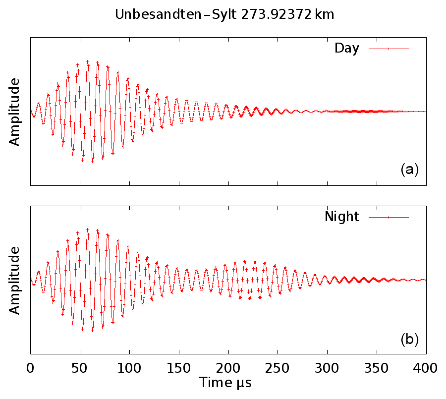
Figure 10 Pulse of the LORAN navigation system received 274 km away from transmitter. In panel (b) taken at 01:00 UTC the D-Layer reflection is clearly visible. It correspondents to a height of about 86 km.

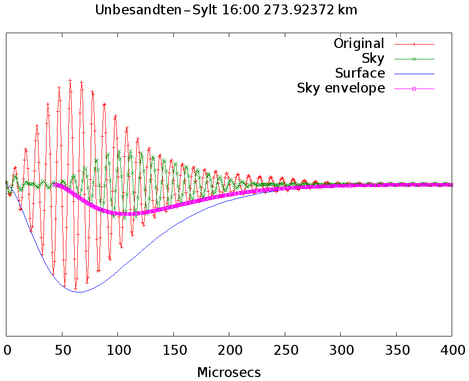
Figure 11 LORAN signal with calculated surface envelope (blue), sky signal (green) and its envelope to estimate the delay against the surface wave, which is here 42 µs.

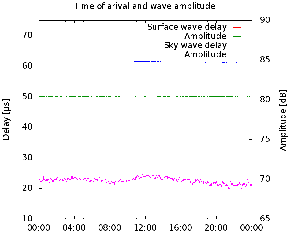
Figure 12 Daily variation of amplitude and signal delay of the emissions from Sylt, 274 km away. Recorded on 26 November 2014. The nominal run time due to the speed of light for this distance is removed but the receiver delay is not removed.

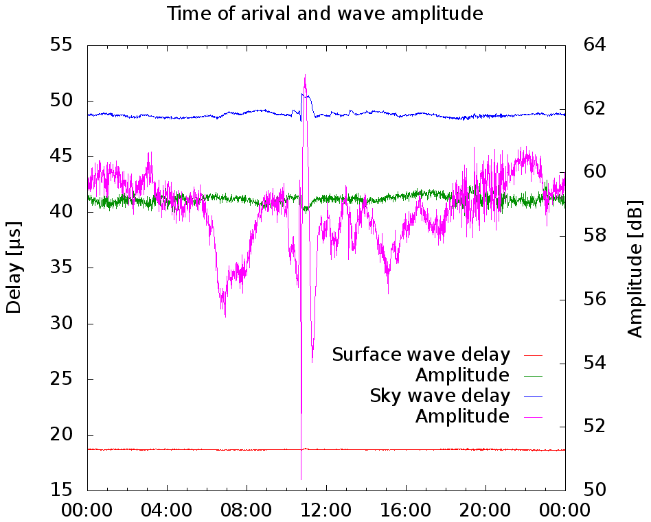
Figure 13 Daily variation of amplitude and signal delay from of the emissions from Lessay, 993 km away. Recorded on 26 November 2014. The nominal run time due to the speed of light for this distance is removed but the receiver delay is not removed.

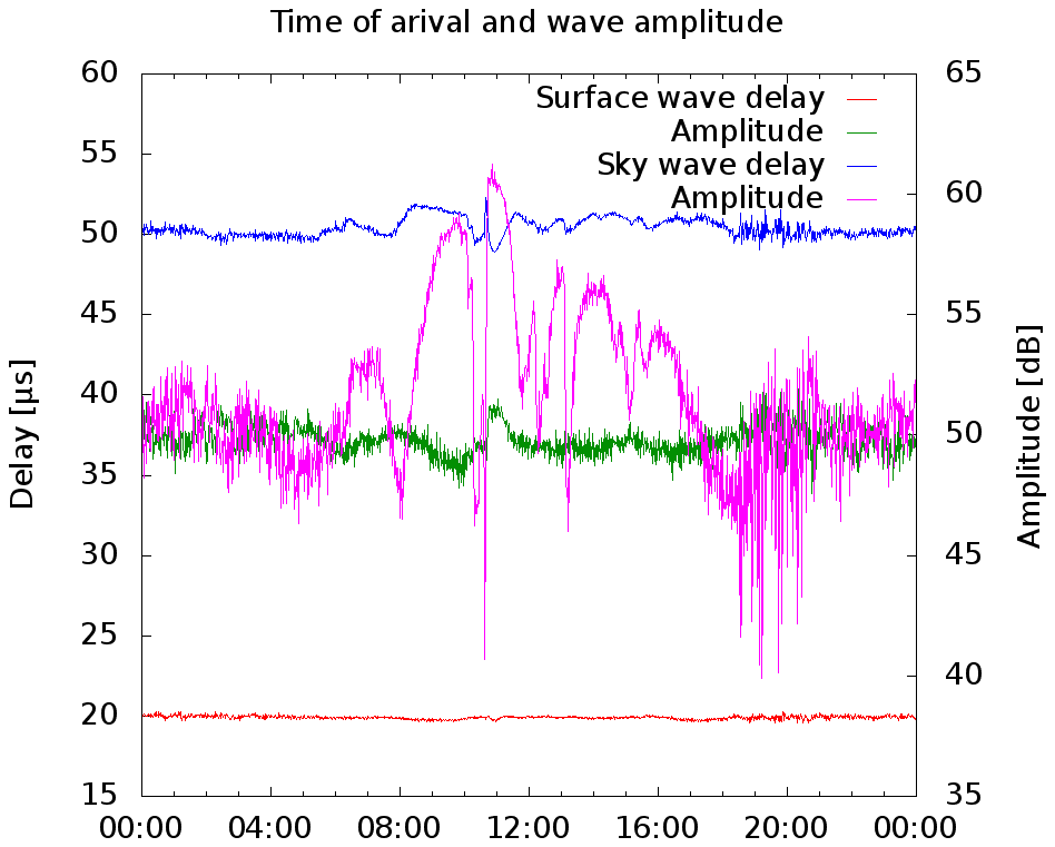
Figure 14 Daily variation of amplitude and signal delay of the emissions from Soustons, 1395 km away. Recorded on 26 November 2014. The nominal run time due to the speed of light for this distance is removed but the receiver delay is not removed.

5 Conclusions

It could be proven that the surface wave is constant both in run time and in amplitude. The daily run time deviation is less than 1 µs even over a distance of 1400 km over land surface. That means that there is a strong evidence that a third wave must exist to explain the midpoint movements in Fig. 8b. It seems also possible that the wave guide propagation model has to be used here in day time. The evaluation of the LORAN pulses clearly shows that waves arrive before the mesospheric echoes, which could be the ones searched for. This is in accordance with C layer publications (Rasmussen et al., 1980; Bertoni et al., 2013) which also point to earlier echos. Since the amplitude of this waves is in the same order of magnitude as the ground wave, when the 1000 km distance is considered, it makes a significant contribution to the reception field strength. The propagation model has to be questioned, as several effects cannot be explained with the used simple approach.

The findings based on SPH regarding trends are still valid. But the direct coupling to the mesosphere must be abandoned. Even the troposphere can have an essential influence onto the observed long wave behavior. Therefore, the SPH series must be considered as one that only reflects integral properties of the hole region from the mesosphere over the stratosphere down to the troposphere.

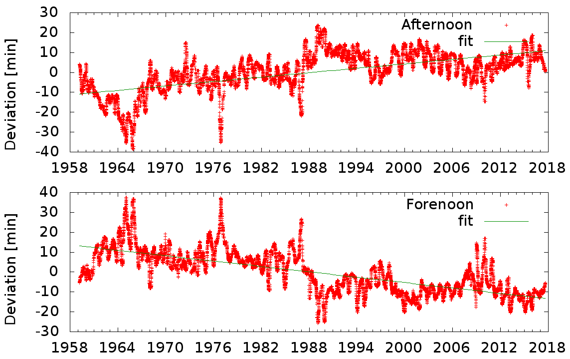
Figure 15 Deviation from the average of the occurrence of the second minimum in the daily Hollingwoth pattern in the morning after sunrise and the second minimum before sunset. The seasonal component is removed as described. The plots are smoothed by a 101 d running median.

However, a simple mathematical approach seems to make sense in order to obtain a statement on long-term behavior. Only the times of occurrence of the extreme values were used. To remove seasonal behavior the whole time series, more then 50 years, were fitted against Eq. (2). with x as running day of the series.

$$\begin{array}{}\text{(2)}& z\left(x\right)={\sum }_{n=\mathrm{1}}^{n=\mathrm{5}}\left[a_n\cos \left({\displaystyle \frac{x}{\mathrm{365.2422}}}\cdot \mathrm{2}\mathit{\pi }n+c_n\right)\right]+d\end{array}$$

This function z(x) was then subtracted from the time series to remove seasonality. As an example, the times of the second minimum after sunrise and the second minimum before sunset are plotted in Fig. 15. The linear fit shows an earlier occurrence of the minimum of 27 min over a period of 60 years in the morning and 22 min in the afternoon. This can be interpreted as an extension of the ionospheric day by 49 min over this long period.