 | 19 Sep 2019
Tidal wind shear observed by meteor radar and comparison with sporadic E occurrence rates based on GPS radio occultation observations
Christina Arras
We analyze tidal (diurnal, semidiurnal, terdiurnal, quarterdiurnal) phases and related wind shear in the mesosphere/lower thermosphere as observed by meteor radar over Collm (51.3∘ N, 13.0∘ E). The wind shear phases are compared with those of sporadic E (Es) occurrence rates, which were derived from GPS radio occultation signal-to-noise ratio (SNR) profiles measured by the COSMIC/FORMOSAT-3 satellites. At middle latitudes Es are mainly produced by wind shear, which, in the presence of a horizontal component of the Earth's magnetic field, leads to ion convergence in the region where the wind shear is negative. Consequently, we find good correspondence between radar derived wind shear and Es phases for the semidiurnal, terdiurnal, and quarterdiurnal tidal components. The diurnal tidal wind shear, however, does not correspond to the Es diurnal signal.
- Article
(3470 KB) - Full-text XML
- BibTeX
- EndNote


In the lower ionospheric E region, shallow regions of high electron density are found, which are called sporadic E (Es) layers. Es layers consist of thin clouds of accumulated ions. They occur mainly at middle latitudes, and they are most frequently found during the summer season (e.g., Arras et al., 2008). Es are generally formed at heights between 90 and 120 km. Their occurrence can be described through the wind shear theory (Whitehead, 1961). According to this theory, Es formation is due to interaction between the metallic ion concentration, the Earth's magnetic field, and the vertical shear of the neutral wind (e.g., Gong et al., 2014). If one neglects diffusion, the neutral gas vertical wind component, and electric forces in the ion momentum budget equation, the vertical ion drift wI becomes (e.g., Haldoupis, 2012; Fytterer et al., 2014; Oikonomou et al., 2014):
Here U and V are the zonal and meridional neutral wind components pointing eastward and northward, respectively, and I is the inclination of the Earth's magnetic field. The parameter is the ratio of the collision frequency ν between the ions and neutrals, and the gyro frequency , where e is the elementary charge, B0 is intensity of the Earth's magnetic field, and mI is the ion mass. Since r≫1 below ∼115 km (Bishop and Earle, 2003), U is more efficiently causing vertical plasma drift than V in the lower E region. Therefore, the second term of Eq. (1) becomes small there, so that mainly the zonal wind U is responsible for the vertical ion drift. Ion accumulation, i.e. the formation of Es, is consequently expected at those altitudes where the vertical gradient of the vertical ion drift is negative (), which in turn corresponds to the region of maximum negative vertical gradient of the zonal wind, i.e. of maximum negative vertical zonal wind shear dU∕dz. Equation (1) is only valid for magnetic middle latitudes (about 20–70∘), because electric forces may be neglected there.
Correspondence between wind shear and Es had been obtained by Chu et al. (2014), who calculated ion flux divergence by using a model based on the WACCM global circulation model, astronomically derived meteoric influx, and winds from the Horizontal Wind Model HWM07 (Drob et al., 2008). They found that wind shear theory satisfactorily explains the summer Es maximum, although their metallic ion distribution also maximises in summer, which is broadly in correspondence with qualitative results by Haldoupis et al. (2007) who compared meteor rates with Es occurrence rates (OR). Shinagawa et al. (2017) analyzed the global distribution of vertical ion convergence based on GAIA Earth system model predictions. They showed that the ion convergence distribution is broadly consistent with Es OR. Liu et al. (2018) found correspondence between Es OR, calculated from Global Positioning System (GPS) radio occultation (RO) data, and wind shear measured with the TIDI instrument (Killeen et al., 2006) on the TIMED satellite.
The dynamics of the lower thermosphere at time scales up to one day are mainly influenced by solar tides, with periods of a solar day and its harmonics (e.g., Forbes, 1995). Their wind amplitudes usually maximize around or above 120 km. In these regions, tidal amplitudes are of the order of magnitude of the mean wind. Shorter period tidal waves often have smaller amplitudes, so that, on a global scale, the major diurnal variability of lower thermosphere winds is due to the diurnal tide (DT, Pancheva et al., 2002), the semidiurnal tide (SDT, Jacobi et al., 1999a, b; Pancheva et al., 2002; Jacobi, 2012), and, to a lesser degree, also to the terdiurnal tide (TDT, Beldon et al., 2006; Fytterer et al., 2013; Lilienthal et al., 2018). Note however, that at higher midlatitudes the DT amplitudes become small compared with SDT ones during most of the year. Owing to its smaller amplitude, the quarterdiurnal tide (QDT) has been analyzed less frequently in the past (Smith et al., 2004), but more recently has attained increasing attention (Liu et al., 2015; Azeem et al., 2016; Jacobi et al., 2017, 2018a, b; Guharay et al., 2018; Gong et al., 2018).
Solar tides are a major source of the vertical wind shear, and the tidal contribution to the overal wind shear is frequently larger than the one of the background wind. Therefore, tide-like structures are also expected in Es occurrence rates. Consequently, the SDT and DT are generally accepted to be the major driver of Es (Mathews, 1998), and they lead to the downward moving tidal signatures in Es ionosonde registrations (e.g., Haldoupis et al., 2006; Haldoupis, 2012). Analyzing GPS Es observations together with meteor radar wind measurements at Collm (51.3∘ N, 13.0∘ E), Arras et al. (2009) could show that during one day Es OR maximize when the zonal wind shear component due to the SDT is negative. More recently, Fytterer et al. (2013) found a clear correspondence between Collm zonal wind shear and Es OR for the 8 h component as well, while Fytterer et al. (2014) showed from comparison of GPS Es RO and modeled wind shear the similarity of the TDT in Es and wind shear on a global scale. Similarly, Jacobi et al. (2018a) recently showed that on a local scale QDT phases agree with negative QDT wind shear phases, and also the global distribution of QDT in Es is related to the one in wind shear. Resende et al. (2018b) modeled the connection of Es and tides, although focusing at the equatorial region, where electric field effects become more important than at middle latitudes.
The Collm meteor radar measures mesospheric and lower thermospheric winds at altitudes of about 80–100 km since summer 2004 (Jacobi et al., 2007, 2009; Lilienthal and Jacobi, 2015). These observations have already been used for comparison with SDT, TDT, and QDT components in Es at these heights (Arras et al., 2009; Fytterer et al., 2013; Jacobi et al., 2018a), but for different time intervals, and without providing an overview of all tidal components together. In particular, the possible correspondence of the DT wind shear over Collm with Es has not yet been considered. Therefore, in this paper we analyze the DT, SDT, TDT and QDT seen in Es, obtained from GPS RO measurements by the FORMOsa SATellite mission-3/Constellation Observing System for Meteorology, Ionosphere and Climate (FORMOSAT-3/COSMIC) at the latitude of Collm and compare Es phases with phases of negative wind shear obtained from the local radar observations at Collm. Since the seasonal cycle of Es and wind shear is different, comparison of amplitudes does not show clear correspondence, so that we restrict ourselves to the discussion of phase similarities. The remainder of the paper is organized as follows. In Sect. 2 the Es detection and the radar wind observations are described. Results of tidal phase analysis and comparison with wind shear phases are presented in Sect. 3. Section 4 concludes the paper.
2.1 Sporadic E occurrence rates
We make use of ionospheric RO measurements by the FORMOSAT-3/COSMIC constellation, which performs observations in both the neutral and ionized atmosphere (Anthes et al., 2008) though a constellation of six low-Earth orbiting (LEO) satellites. During each occultation, signals of the rising or setting GPS satellites are received by a LEO satellite. When the signals pass the atmosphere/ionosphere of the Earth, they are influenced in particular by the ionospheric electron density, which cause refraction and degradation of the GPS waves. This effect can be utilized to obtain information about the ionosphere. Observation of the neutral atmosphere is also possible, but is not the topic of this study. Detailed information on the RO technique principles is provided by Hajj et al. (2002) and Kursinski et al. (1997).
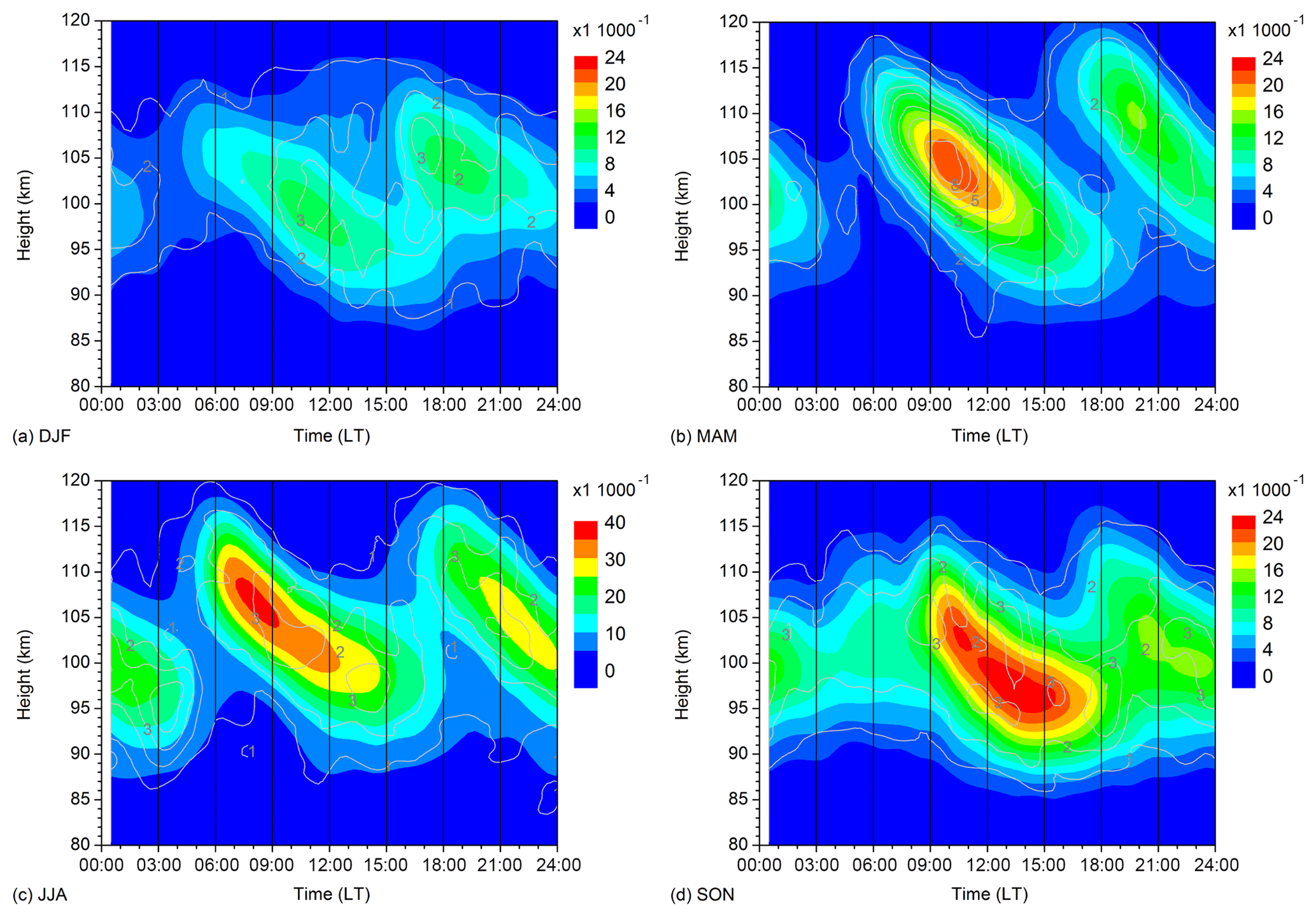
Figure 1Zonal and seasonal mean Es occurrence rates for (a) DJF, (b) MAM, (c) JJA, (d) SON. Data are averages over 2007–2016. Note the different scaling for the summer OR. The grey contour lines show standard deviations calculated from wind shear values for single years.
To derive information on Es from RO, we use the Signal-to-Noise ratio (SNR) profiles of the GPS L1 phase measurements. The SNR is very sensitive to vertical gradients of the electron density, which occur within Es layers. These localized electron density variations lead to phase fluctuations of the GPS signal, which are observed as changes of the received signal strength (Hajj et al., 2002). The basic signal power differs among ROs; therefore the SNR profiles are normalized before they are analyzed. In those cases when no ionospheric disturbances occur, the SNR value is almost constant above 35 km altitude. We analyze the vertical profile of the standard deviation of the SNR. If the SNR exceeds an empirically found threshold of 0.2, the profile is considered to be disturbed. If large standard deviation values occur that are concentrated within a layer of less than 10 km thickness, we assume that the respective SNR profile disturbance is owing to an Es layer. The height where the SNR value most strongly deviates from the mean of the SNR profile is taken as the Es layer altitude, as has been been validated by comparisons with ionosonde observations (Arras and Wickert, 2018; Resende et al., 2018a). The Es OR is simply calculated by the number of Es registrations in a given time, height, and latitude interval divided by the number of RO in that time and latitude interval. The method to derive Es OR from RO records was described by Arras and Wickert (2018).
Figure 1 shows 2007–2016 mean diurnal cycles of Es OR within a 10∘ latitude window centered at 51.3∘ N, and within a 10 km height window each. Data from all longitudes are used. We show seasonal means for December–February (DJF), March–May (MAM), June–August (JJA) and September–November (SON), with the respective standard deviations calculated from the OR data of single years added as grey contours. Maximum OR are found at altitudes slightly above 100 km. OR maximize in summer, which is thought to be owing to increased meteor influx during that season (Haldoupis et al., 2007), although Chu et al. (2014) claimed that wind shear theory gives an explanation for this maximum, too. We note that the diurnal variability of Es mainly contains a diurnal and semidiurnal component. The quarterdiurnal and terdiurnal components, however, although being weaker, are also included in the spectrum as was shown by Jacobi et al. (2018a) and Fytterer et al. (2013).
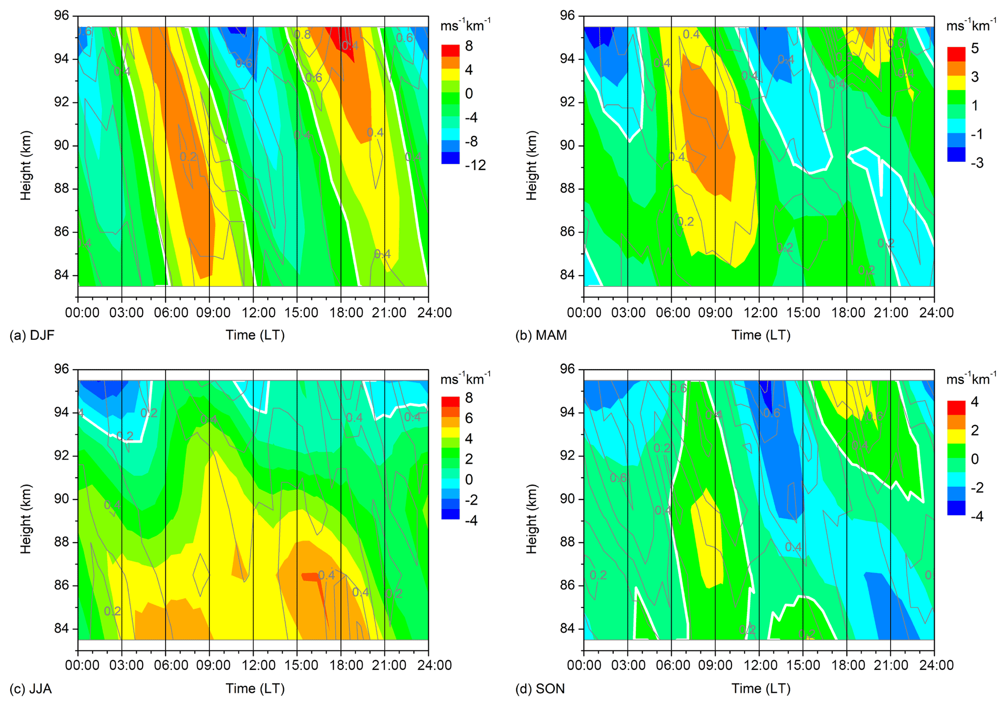
Figure 2Seasonal mean zonal wind shear over Collm for (a) DJF, (b) MAM, (c) JJA, (d) SON. Data are averages over 2007–2016. The zero line is highlighted. Note the different scaling of the respective panels. The grey contour lines show standard deviations in calculated from wind shear values for single years.
The tidal components of Es OR are calculated with a modeled least-squares fit including mean Es0, 6, 8, 12, and 24 h components:
with t as the time and Pi as the above mentioned periods. The coefficients ai and bi are determined through minimizing . The phases Ti of Es OR are derived from ai and bi as
2.2 Collm mesosphere/lower thermosphere wind shear
At Collm (51.3∘ N, 13.0∘ E), a SKiYMET meteor radar is operated since summer 2004. The radar operates on 36.2 MHz in a quasi all-sky configuration, and the main parameter observed are the MLT radial winds determined from the Doppler shift of individual meteor trails. Details of the radar system and the radial wind determination principle can be found in Jacobi (2012), Stober et al. (2012), and Lilienthal and Jacobi (2015). During 2015 the radar was upgraded by increasing the peak power, and replacing the until then used Yagi antennas by crossed dipoles, while maintaining the transmit frequency (Stober et al., 2017). The heights of the individual meteor trail reflections vary between about 75 and 110 km, and the maximum meteor count rate is found at an altitude slightly below 90 km (e.g., Stober et al., 2008).
The data are binned here in 6 different not overlapping height gates that are centered at 82, 85, 88, 91, 94, and 98 km. The hourly mean reflection height may slightly deviate from the nominal heights due to the uneven height distribution of meteors within each gate (Jacobi, 2012), and in particular the real mean height of the uppermost height gate is close to 97 km rather than 98 km so that we use this height as reference altitude for the uppermost gate. Hourly mean horizontal wind values are calculated from the individual radial winds within one height gate using a least squares fit of the horizontal wind components to the raw data. This is done under the assumption that vertical winds are negligibly small (Hocking et al., 2001). As in Arras et al. (2009), Fytterer et al. (2013), and Jacobi et al. (2018a) hourly values of the zonal wind shear are calculated from adjacent height gates. The reference height for shear values is attributed to the center between the nominal heights of the height gates.
Figure 2 shows 2007–2016 seasonal mean diurnal cycles of zonal wind shear over Collm. Again, the figure shows means for DJF, MAM, JJA, and SON, with the respective standard deviations (in ) calculated from the shear data of single years added as grey contours. The zonal wind shear maximizes at more than ±8 m s−1 in winter, similar to the values shown by Arras et al. (2009) for January 2007. Clearly, the main contribution to zonal wind and wind shear variability in winter is due to the SDT. However, during the equinoxes the diurnal cycle below about 90 km is more dominated by the diurnal component. In summer, the wind shear is mainly positive, which is due to the strong positive gradient of the zonal prevailing wind in combination with small tidal amplitudes (Schminder et al., 1997; Manson et al., 2003; Jacobi et al., 2009; Jacobi, 2012). Therefore, considerable summer tidal amplitudes are only observed at greater altitudes and negative wind shear with a semidiurnal diurnal cycle can be seen only above ∼93 km. Therfore, ion accumulation and thus Es formation is not supported below ∼93 km, which can be see in Fig. 1, where summer Es are present at greater altitudes than Es during the other seasons. This is in accordance with results, e.g., by Chu et al. (2014) who also showed the higher summer Es altitudes.
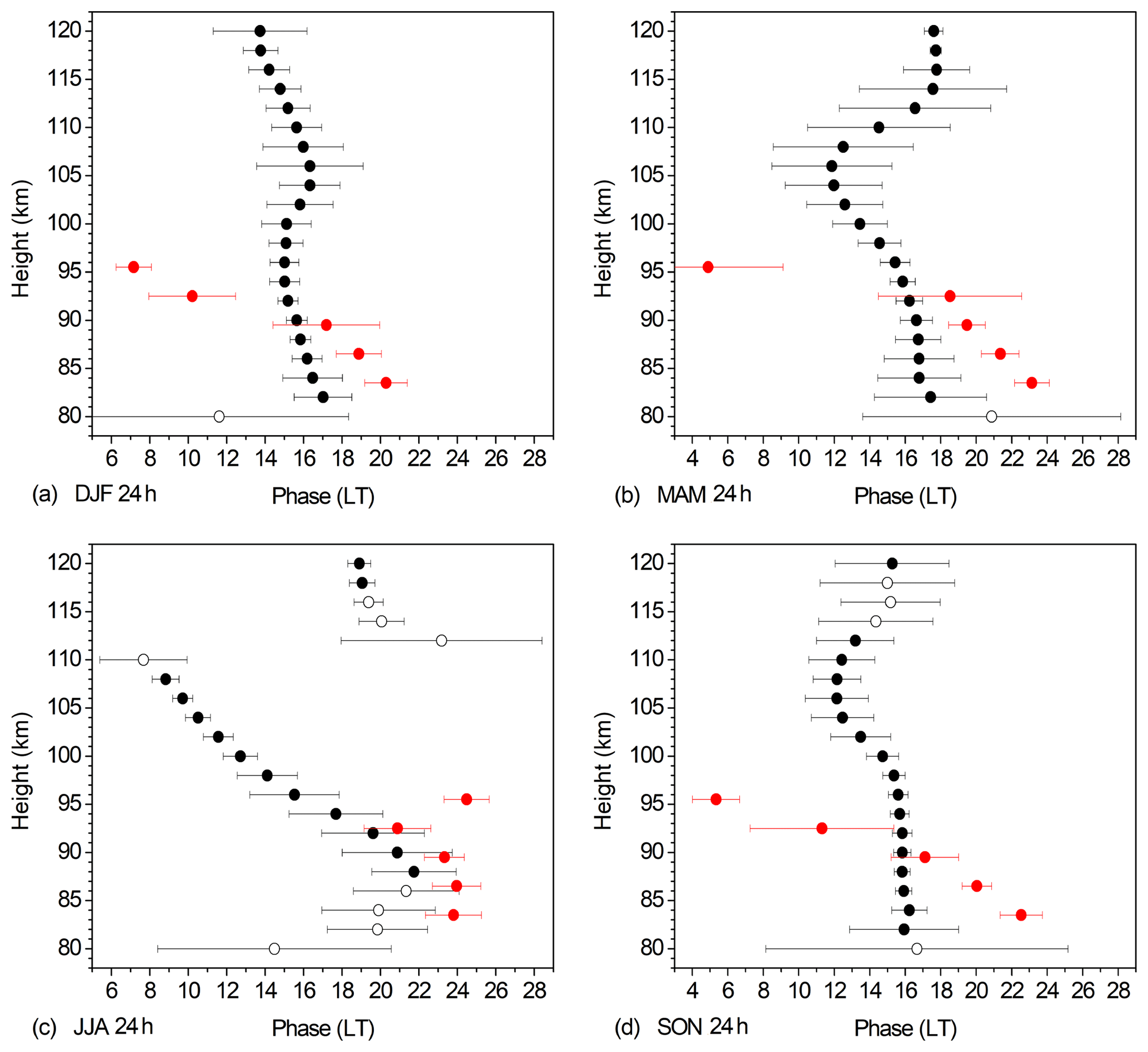
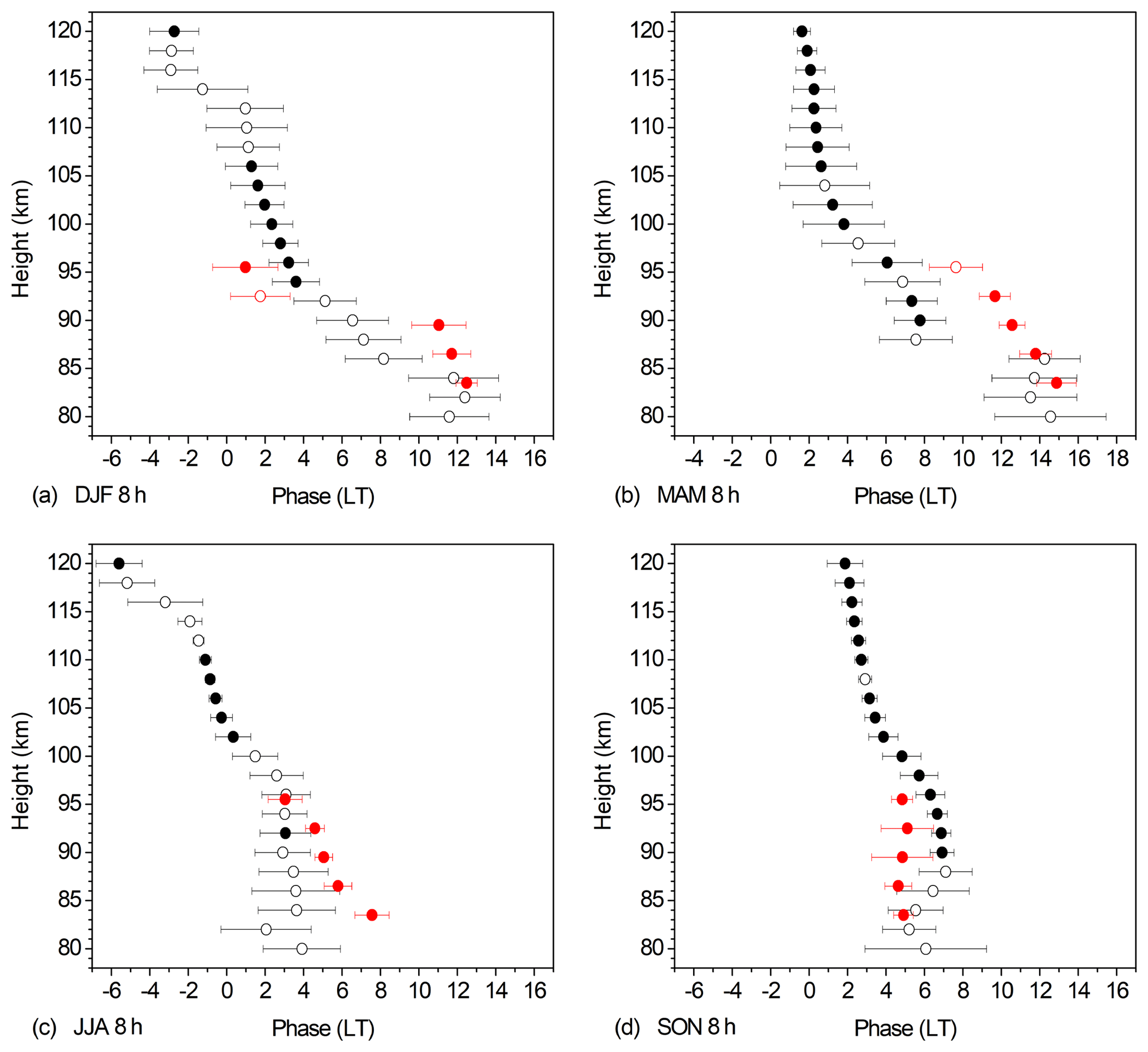
Figure 3Zonal and seasonal mean Es DT phases at 51∘ N for (a) DJF, (b) MAM, (c) JJA, (d) SON. Data are averages over 2007–2016. Collm wind shear phases acccording to Eq. (4) are added in red. Solid symbols denote oscillations significant at the 5 % level according to a t test. The error bars show standard deviations calculated from phases for single years.
The tidal components of zonal wind shear are calculated with a modeled least-squares fit according to Eq. (3). The wind shear phases are:
similar to Eq. (3), but since here we define the phases as the local time of maximum negative wind shear, the Pi∕2-term is added to the right hand side of Eq. (4).
One can clearly see from Figs. 1 and 2 that the seasonal cycle of Es amplitudes does not correspond with the one of zonal wind shear below 100 km. Es maximize in summer, while the largest shear amplitudes are found in winter. The discrepancy arises because Es OR amplitudes are not only influenced by wind shear, but also by background Es OR, which are dependent on meteor influx and background ionization in the course of a day. Therefore, in the following we only compare phases of the 24, 12, 8, and 6 h components of the Es OR and the negative wind shear in order to check whether ion accumulation actually take place at the convergence nodes of vertical ion drift forced by vertical wind shear. Note that the results for the QDT phases have already been presented in Jacobi et al. (2018a), but are repeated here for the sake of completeness.
The radar observations of wind shear are only available at altitudes up to about 95 km. Therefore, direct comparison between wind shear and Es phases is not possible above that height. However, if we find a correspondence between Es and wind shear at lower altitudes for some tidal components, this may be considered as an indication that above 100 km the Es diurnal cycle is also connected with tidal wind shear, although this cannot be considered as a real proof for such a hypothesis.
3.1 Diurnal tide
Ground-based and satellite observations as well as model results show that the migrating DT amplitudes maximize at or equatorward of 30∘ latitude (Hagan et al., 1997; Manson et al., 2002; Pancheva et al., 2002; Portnyagin, 2006; Wu et al., 2008). Poleward of 50∘ the DT wind amplitudes are usually much smaller than the SDT ones, which also has been frequently shown by radar observations (Xu et al., 2012; Jacobi, 2012). Therefore it is not expected that the relatively strong DT signature in Es as is seen in Fig. 1 is soleyly due to a strong wind shear DT. One may rather assume that the diurnal cycle of background ionization may enhance the daytime Es OR and therefore leads to a DT signature in Es.
Zonal and seasonal mean Es phases at 51∘ N of the diurnal component for four seasons are shown in Fig. 3. Data are averages over 2007–2016. Collm DT wind shear phases according to Eq. (4) are added in red. Solid symbols denote oscillations significant at the 5 % level according to a t test. The error bars show standard deviations calculated from phases for single years. During most seasons, the Es phase is largely constant with height. This would be consistent with the diurnal maximum of Es owing to the general diurnal change of ionization. The Es phases do not agree with wind shear ones during most of the year, except for summer at altitudes below about 95 km. However, it is not clear whether this correspondence may be due to coincidence. Although this does not exclude a wind shear effect on Es, during most seasons a clear difference of the phase structure shows that there is another effect on the diurnal Es signature. The general disagreement between Es and wind shear phases therefore leads to the conclusion that the main part of the diurnal cycle of Es is most probably not due to the diurnal wind shear cycle and not related to the wind shear DT.
3.2 Semidiurnal tide
Globally, the SDT extends more into the northern winter hemisphere than the DT (Hagan et al., 1995; Pancheva et al., 2002; Portnyagin, 2006), and the SDT is the strongest tidal component at 50–60∘ latitude. Its amplitude at 90–100 km maximises during winter and autumn, which was frequently shown from ground based and space borne observations (Manson and Meek, 1984; Manson et al., 2003; Burrage et al., 1995; Schminder et al., 1997; Xu et al., 2012; Jacobi, 2012; Pokhotelov et al., 2018), but in the thermosphere the SDT amplitudes are large in summer as well (Pancheva et al., 2009). Zonal and seasonal mean phases at 51∘ N of the Es semidiurnal component for four seasons are shown in Fig. 4. Data are again averages over 2007–2016, together with Collm SDT wind shear phases according to Eq. (4).
Es phases broadly agree with wind shear ones in winter and especially in spring. In particular, their vertical gradients agree with each other. This is in agreement with Chu et al. (2014) who found from comparison of the diurnal cycle of Es occurrence and wind shear derived from the empirical HWM07 model that these are broadly in agreement for the SDT. Note that the SDT phases do not vary strongly from year to year, so that comparison of an empirical climatology and observed Es phases will provide reasonable results.
There is a small but significant difference in winter. This might be due to a nonmigrating SDT component which could lead to a difference of local and zonal mean phases. However, nonmigrating SDT amplitudes are not large, as was shown by Oberheide et al. (2007) from TIDI satellite observations. Longitudinal phase differences are of the order of 1 h (Jacobi et al., 1999a), but the Collm SDT phases had been shown to be rather close to the zonal mean (Cierpik et al., 2003). Still, however, this effect may explain the difference between wind shear and Es phases in Fig. 4a.
In summer there is correspondence between SDT wind shear and Es phases only at ∼95 km, and in autumn this is only the case at altitudes above 90 km. However, in autumn at lower altitudes Es 12 h oscillations are not significant anyway, which may be due to the small SDT zonal wind shear amplitudes. Also Chu et al. (2014) did not observe good correspondence between Es and wind shear at lower altitudes in summer. Figure 2 shows that below about 90 km the autumn diurnal wind shear is dominated by the DT, but not by a semidiurnal component. In summer, SDT wind amplitudes are small at heights below 90 km, and the vertical wavelength is large (Jacobi, 2012). Therefore, the SDT wind shear amplitude at these heights is generally small in summer. Taking into account that the background wind shear is strongly positive in the upper mesosphere, wind shear effects on the Es diurnal cycle, if any, are expected only for the upper radar height gates. Indeed, Fig. 2 shows negative wind shear only for the uppermost height gates, which corresponds to the similarity of Es and wind shear phases at about 95 km, but not below that height, which is seen in Fig. 4c.
3.3 Terdiurnal tide
Hints for terdiurnal signatures in Es were first reported by Szuszczewicz et al. (1995), in a case study by Haldoupis et al. (2004) in ionosonde critical frequencies at Milos (36.7∘ N) and Rome (41.9∘ N), and by Haldoupis and Pancheva (2006) in a more systematic study. Radar observations at Collm and other sites at similar latitude had shown that the TDT maximizes at equinoxes (Beldon et al., 2006; Jacobi and Fytterer, 2012). Consequently, maximum TDT Es amplitudes at 50∘ N derived from GPS RO are also found during these seasons (Fytterer et al., 2013). During summer, the Es TDT is weaker, although Oikonomou et al. (2014) found a TDT only during that season.
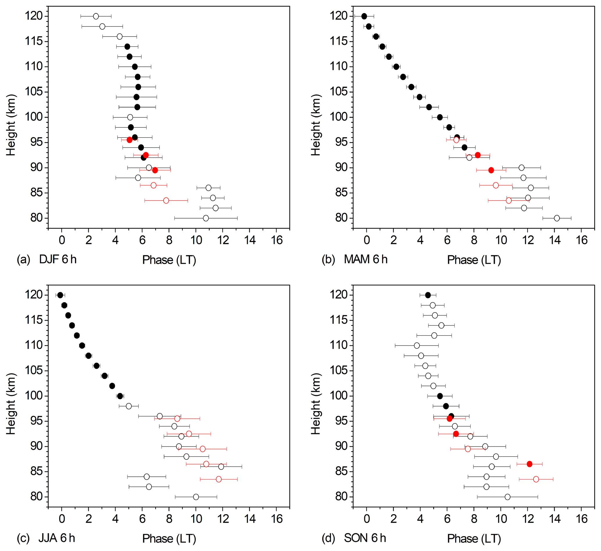
Figure 6As in Fig. 3, but for the QDT. These phases have also been shown in Jacobi et al. (2018a).
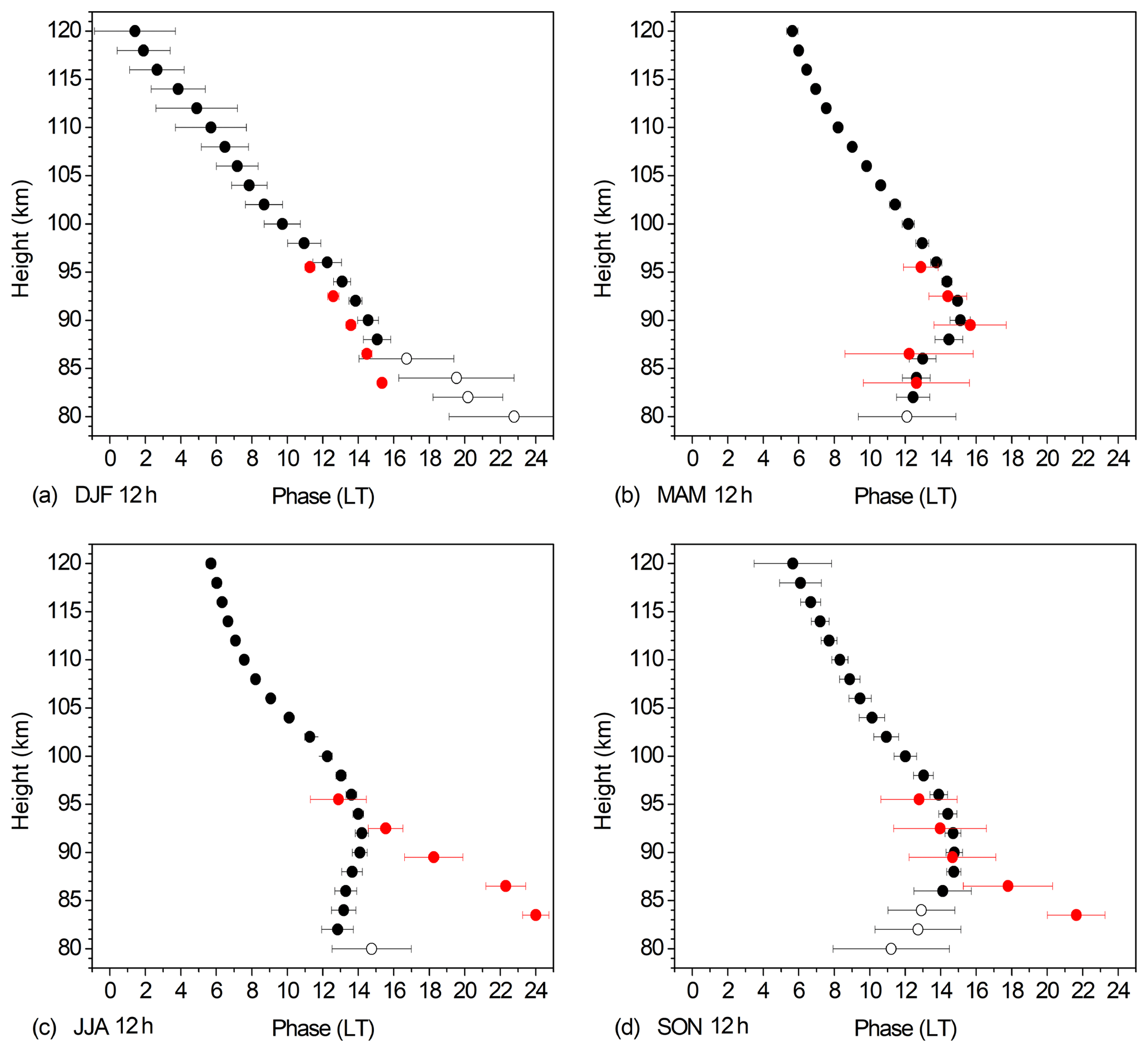
Zonal and seasonal mean Es OR phases at 51∘ N of the TDT for four seasons are shown in Fig. 5. As in Figs. 3 and 4 the data are averages over 2007–2016, and Collm wind shear phases according to Eq. (4) are added in red. The data represent an update of the results for 2007–2010 that were presented by Fytterer et al. (2013). Note that the TDT maximizes near equinoxes (Jacobi, 2012; Jacobi and Fytterer, 2012; Fytterer et al., 2013), and correspondingly the Es TDT are more significant then.
We note a correspondence of Es OR phases and Collm zonal negative wind shear, especially concerning their changes with height. During winter, at 95 km Es and wind shear phases fit within their standard deviation, while there are some differences below, however, at these heights the Es TDT is not significant. During spring, there is a time shift visible between wind shear and Es phases above 90 km. In the lower part the phases are the same, but the Es TDT is not significant there. We conclude that notwithstanding the larger TDT amplitudes in spring, a clear correspondence of TDT wind shear and Es is not seen then, apart from the vertical phase gradients that are similar.
As with the summer SDT, the Es and wind shear TDT phases during summer only correspond at 95 km. This can again be explained by the positive wind shear provided by the background wind, similar as with the SDT. Note, however, if one extrapolates the wind shear phases, they would fit the Es ones also slightly above 95 km. During autumn, there is a correspondence between Es and wind shear TDT phases. However, in autumn the vertical phase gradient is close to zero, i.e. the wave is evanescent as has been shown already by Jacobi (2012). Therefore the wind shear TDT amplitudes are small and the correspondence with Es phases may be due to coincidence. Nevertheless, given the overall similarity of wind shear and Es phases we may conclude that the wind shear mechanism plays a role in forming the TDT in Es, although the correspondence is not that clear than the one of the SDT components.
3.4 Quarterdiurnal tide
There are not many reports on a 6 h component in Es. Some publications report that no QDT have been found in ionospheric records (e.g., Cyprus, 35∘ N, 33∘ E, Oikonomou et al., 2014). However, 6 h tidal signatures have been observed by incoherent scatter observations in lower ionospheric Es parameters over Arecibo (18.3∘ N, Tong et al., 1988; Morton et al., 1993), and QDT signatures were found in summer ionograms performed by Lee et al. (2003) at 24.3∘ N. A study based on GPS RO has recently been performed by Jacobi et al. (2018a).
Zonal and seasonal mean Es phases at 51∘ N of the QDT for four seasons are shown in Fig. 6. Again, data are averages over 2007–2016, and wind shear phases are added. The data are the same as were shown already in Jacobi et al. (2018a), so that they are only briefly discussed here. Phases of the Es OR QDT agree very well with wind shear QDT phases during each season, and given the generally small QDT amplitudes (Jacobi et al., 2017) the correspondence is striking, particularly in summer when the TDT is not significant. We may conclude that the wind shear mechanism is most probably responsible for the 6 h oscillation in Es.
Tidal phases from lower thermosphere meteor radar zonal wind shear measurements at 51.3∘ N are analyzed together with Es OR phases at the same latitude. The seasonal cycle of Es amplitudes is influenced by the Es seasonal cycle with maximum in summer. Consequently, there is no correspondence between tidal amplitudes in Es and wind shear tidal amplitudes, and our analysis is limited to the comparison of phases.
Phases of SDT, TDT and QDT fit reasonably well during most seasons. This means that tides seen in Es are probably at least partly due to neutral zonal wind shear in the presence of a northward component of the Earth´s magnetic field. The diurnal component of Es OR diurnal variability, however, does not fit to zonal wind shear phases during most seasons, and is therefore probably not primarily owing to the neutral wind DT.
Radio occultation data are freely available from UCAR on http://cdaac-www.cosmic.ucar.edu/cdaac/products.html, last access: 26 September 2018. Collm radar wind shears are available from the corresponding author on request.
CJ performed Collm radar wind measurements and analyses, as well as the tidal analyses based on GPS Es, which were analyzed by CA. The paper was written jointly by CJ and CA.
The authors declare that they have no conflict of interest.
This article is part of the special issue “Kleinheubacher Berichte 2018”. It is a result of the Kleinheubacher Tagung 2018, Miltenberg, Germany, 24–26 September 2018.
The provision of FORMOSAT-3/COSMIC data by University Corporation for Atmospheric Research is gratefully acknowledged. Christoph Jacobi acknowledges support through the Deutsche Forschungsgemeinschaft (DFG) under grants JA 836/30-1 and JA 836/34-1. Christina Arras acknowledges support by the DFG Priority Program DynamicEarth, SPP 1788.
This paper was edited by Ralph Latteck and reviewed by Laysa Resende and one anonymous referee.
Anthes, R. A., Bernhardt, P. A., Chen, Y., Cucurull, L., Dymond, K. F., Ector, D., Healy, S. B., Ho, S.-P., Hunt, D. C., Kuo, Y.-H., Liu, H., Manning, K., McCormick, C., Meehan, T. K., Randel, W. J., Rocken, C., Schreiner, W. S., Sokolovskiy, S. V., Syndergaard, S., Thompson, D. C., Trenberth, K. E., Wee, T.-K., Yen, N. L., and Zeng, Z.: The COSMIC/FORMOSAT-3 Mission: Early Results, B. Am. Meteorol. Soc., 89, 313–334, https://doi.org/10.1175/BAMS-89-3-313, 2008. a
Arras, C. and Wickert, J.: Estimation of ionospheric sporadic E intensities from GPS radio occultation measurements, J. Atmos. Sol.-Terr. Phy., 171, 60–63, https://doi.org/10.1016/j.jastp.2017.08.006, 2018. a, b
Arras, C., Wickert, J., Beyerle, G., Heise, S., Schmidt, T., and Jacobi, C.: A global climatology of ionospheric irregularities derived from GPS radio occultation, Geophys. Res. Lett., 35, L14809, https://doi.org/10.1029/2008GL034158, 2008. a
Arras, C., Jacobi, C., and Wickert, J.: Semidiurnal tidal signature in sporadic E occurrence rates derived from GPS radio occultation measurements at higher midlatitudes, Ann. Geophys., 27, 2555–2563, https://doi.org/10.5194/angeo-27-2555-2009, 2009. a, b, c, d
Azeem, I., Walterscheid, R. L., Crowley, G., Bishop, R. L., and Christensen, A. B.: Observations of the migrating semidiurnal and quaddiurnal tides from the RAIDS/NIRS instrument, J. Geophys. Res.-Space Phys., 121, 4626–4637, https://doi.org/10.1002/2015JA022240, 2016. a
Beldon, C., Muller, H., and Mitchell, N.: The 8-hour tide in the mesosphere and lower thermosphere over the UK, 1988–2004, J. Atmos. Sol.-Terr. Phy., 68, 655–668, https://doi.org/10.1016/j.jastp.2005.10.004, 2006. a, b
Bishop, R. L. and Earle, G. D.: Metallic ion transport associated with midlatitude intermediate layer development, J. Geophys. Res.-Space Phys., 108, SIA 3–1–SIA 3–8, https://doi.org/10.1029/2002JA009411, 2003. a
Burrage, M. D., Hagan, M. E., Skinner, W. R., Wu, D. L., and Hays, P. B.: Long-term variability in the solar diurnal tide observed by HRDI and simulated by the GSWM, Geophys. Res. Lett., 22, 2641–2644, https://doi.org/10.1029/95GL02635, 1995. a
Chu, Y. H., Wang, C. Y., Wu, K. H., Chen, K. T., Tzeng, K. J., Su, C. L., Feng, W., and Plane, J. M. C.: Morphology of sporadic E layer retrieved from COSMIC GPS radio occultation measurements: Wind shear theory examination, J. Geophys. Res.-Space Phys., 119, 2117–2136, https://doi.org/10.1002/2013JA019437, 2014. a, b, c, d, e
Cierpik, K. M., Forbes, J. M., Miyahara, S., Miyoshi, Y., Fahrutdinova, A., Jacobi, C., Manson, A., Meek, C., Mitchell, N. J., and Portnyagin, Y.: Longitude variability of the solar semidiurnal tide in the lower thermosphere through assimilation of ground- and space-based wind measurements, J. Geophys. Res.-Space Phys., 108, 1202, https://doi.org/10.1029/2002JA009349, 2003. a
Drob, D. P., Emmert, J. T., Crowley, G., Picone, J. M., Shepherd, G. G., Skinner, W., Hays, P., Niciejewski, R. J., Larsen, M., She, C. Y., Meriwether, J. W., Hernandez, G., Jarvis, M. J., Sipler, D. P., Tepley, C. A., O'Brien, M. S., Bowman, J. R., Wu, Q., Murayama, Y., Kawamura, S., Reid, I. M., and Vincent, R. A.: An empirical model of the Earth's horizontal wind fields: HWM07, J. Geophys. Res.-Space Phys., 113, https://doi.org/10.1029/2008JA013668, 2008. a
Forbes, J. M.: Tidal and Planetary Waves, pp. 67–87, American Geophysical Union (AGU), Washington, D.C., https://doi.org/10.1029/GM087p0067, 1995. a
Fytterer, T., Arras, C., and Jacobi, C.: Terdiurnal signatures in sporadic E layers at midlatitudes, Adv. Radio Sci., 11, 333–339, https://doi.org/10.5194/ars-11-333-2013, 2013. a, b, c, d, e, f, g, h
Fytterer, T., Arras, C., Hoffmann, P., and Jacobi, C.: Global distribution of the migrating terdiurnal tide seen in sporadic E occurrence frequencies obtained from GPS radio occultations, Earth Planets Space, 66, 1–9, https://doi.org/10.1186/1880-5981-66-79, 2014. a, b
Gong, Y., Zhou, Q., and Zhang, S.: Numerical and observational study of ion layer formation at Arecibo, in: XXXIth URSI General Assembly, Beijing, China, https://doi.org/10.1109/URSIGASS.2014.6929732, 2014. a
Gong, Y., Ma, Z., Lv, X., Zhang, S., Zhou, Q., Aponte, N., and Sulzer, M.: A Study on the Quarterdiurnal Tide in the Thermosphere at Arecibo During the February 2016 Sudden Stratospheric Warming Event, Geophys. Res. Lett., 45, 13142–13149, https://doi.org/10.1029/2018GL080422, 2018. a
Guharay, A., Batista, P. P., Buriti, R. A., and Schuch, N. J.: On the variability of the quarter-diurnal tide in the MLT over Brazilian low-latitude stations, Earth Planets Space, 70, 140, https://doi.org/10.1186/s40623-018-0910-9, 2018. a
Hagan, M. E., Forbes, J. M., and Vial, F.: On modeling migrating solar tides, Geophys. Res. Lett., 22, 893–896, https://doi.org/10.1029/95GL00783, 1995. a
Hagan, M. E., McLandress, C., and Forbes, J. M.: Diurnal tidal variability in the upper mesosphere and lower thermosphere, Ann. Geophys., 15, 1176–1186, https://doi.org/10.1007/s00585-997-1176-x, 1997. a
Hajj, G., Kursinski, E., Romans, L., Bertiger, W., and Leroy, S.: A technical description of atmospheric sounding by GPS occultation, J. Atmos. Sol.-Terr. Phy., 64, 451–469, https://doi.org/10.1016/S1364-6826(01)00114-6, 2002. a, b
Haldoupis, C.: Midlatitude Sporadic E. A Typical Paradigm of Atmosphere-Ionosphere Coupling, Space Sci. Rev., 168, 441–461, https://doi.org/10.1007/s11214-011-9786-8, 2012. a, b
Haldoupis, C. and Pancheva, D.: Terdiurnal tidelike variability in sporadic E layers, J. Geophys. Res.-Space Phys., 111, A07303, https://doi.org/10.1029/2005JA011522, 2006. a
Haldoupis, C., Pancheva, D., and Mitchell, N. J.: A study of tidal and planetary wave periodicities present in midlatitude sporadic E layers, J. Geophys. Res.-Space Phys., 109, A02302, https://doi.org/10.1029/2003JA010253, 2004. a
Haldoupis, C., Meek, C., Christakis, N., Pancheva, D., and Bourdillon, A.: Ionogram height–time–intensity observations of descending sporadic E layers at mid-latitude, J. Atmos. Sol.-Terr. Phy., 68, 539–557, https://doi.org/10.1016/j.jastp.2005.03.020, 2006. a
Haldoupis, C., Pancheva, D., Singer, W., Meek, C., and MacDougall, J.: An explanation for the seasonal dependence of midlatitude sporadic E layers, J. Geophys. Res.-Space Phys., 112, A06315, https://doi.org/10.1029/2007JA012322, 2007. a, b
Hocking, W., Fuller, B., and Vandepeer, B.: Real-time determination of meteor-related parameters utilizing modern digital technology, J. Atmos. Sol.-Terr. Phy., 63, 155–169, https://doi.org/10.1016/S1364-6826(00)00138-3, 2001. a
Jacobi, C.: 6 year mean prevailing winds and tides measured by VHF meteor radar over Collm (51.3∘ N, 13.0∘ E), J. Atmos. Sol.-Terr. Phy., 78–79, 8–18, https://doi.org/10.1016/j.jastp.2011.04.010, 2012. a, b, c, d, e, f, g, h, i
Jacobi, Ch. and Fytterer, T.: The 8-h tide in the mesosphere and lower thermosphere over Collm (51.3∘ N; 13.0∘ E), 2004–2011, Adv. Radio Sci., 10, 265–270, https://doi.org/10.5194/ars-10-265-2012, 2012. a, b
Jacobi, C., Portnyagin, Y., Solovjova, T., Hoffmann, P., Singer, W., Fahrutdinova, A., Ishmuratov, R., Beard, A., Mitchell, N., Muller, H., Schminder, R., Kürschner, D., Manson, A., and Meek, C.: Climatology of the semidiurnal tide at 52–56∘ N from ground-based radar wind measurements 1985–1995, J. Atmos. Sol.-Terr. Phy., 61, 975–991, https://doi.org/10.1016/S1364-6826(99)00065-6, 1999a. a, b
Jacobi, C., Portnyagin, Y., Solovjova, T., Hoffmann, P., Singer, W., Kashcheyev, B., Oleynikov, A., Fahrutdinova, A., Solntsev, R., Beard, A., Mitchell, N., Muller, H., Schminder, R., and Kürschner, D.: Mesopause region semidiurnal tide over Europe as seen from ground-based wind measurements, Adv. Space Res., 24, 1545–1548, https://doi.org/10.1016/S0273-1177(99)00878-9, 1999b. a
Jacobi, C., Fröhlich, K., Viehweg, C., Stober, G., and Kürschner, D.: Midlatitude mesosphere/lower thermosphere meridional winds and temperatures measured with meteor radar, Adv. Space Res., 39, 1278–1283, https://doi.org/10.1016/j.asr.2007.01.003, 2007. a
Jacobi, C., Arras, C., Kürschner, D., Singer, W., Hoffmann, P., and Keuer, D.: Comparison of mesopause region meteor radar winds, medium frequency radar winds and low frequency drifts over Germany, Adv. Space Res., 43, 247–252, https://doi.org/10.1016/j.asr.2008.05.009, 2009. a, b
Jacobi, C., Krug, A., and Merzlyakov, E.: Radar observations of the quarterdiurnal tide at midlatitudes: Seasonal and long-term variations, J. Atmos. Sol.-Terr. Phy., 163, 70–77, https://doi.org/10.1016/j.jastp.2017.05.014, 2017. a, b
Jacobi, C., Arras, C., Geißler, C., and Lilienthal, F.: Quarterdiurnal signature in sporadic E occurrence rates and comparison with neutral wind shear, Ann. Geophys. Discuss., https://doi.org/10.5194/angeo-2018-125, in review, 2018a. a, b, c, d, e, f, g, h, i
Jacobi, C., Geißler, C., Lilienthal, F., and Krug, A.: Forcing mechanisms of the 6 h tide in the mesosphere/lower thermosphere, Adv. Radio Sci., 16, 141–147, https://doi.org/10.5194/ars-16-141-2018, 2018b. a
Killeen, T. L., Wu, Q., Solomon, S. C., Ortland, D. A., Skinner, W. R., Niciejewski, R. J., and Gell, D. A.: TIMED Doppler Interferometer: Overview and recent results, J. Geophys. Res.-Space Phys., 111, https://doi.org/10.1029/2005JA011484, 2006. a
Kursinski, E. R., Hajj, G. A., Schofield, J. T., Linfield, R. P., and Hardy, K. R.: Observing Earth's atmosphere with radio occultation measurements using the Global Positioning System, J. Geophys. Res.-Atmos., 102, 23429–23465, https://doi.org/10.1029/97JD01569, 1997. a
Lee, C.-C., Liu, J.-Y., Pan, C.-J., and Hsu, H.-H.: The intermediate layers and associated tidal motions observed by a digisonde in the equatorial anomaly region, Ann. Geophys., 21, 1039–1045, https://doi.org/10.5194/angeo-21-1039-2003, 2003. a
Lilienthal, F. and Jacobi, Ch.: Meteor radar quasi 2-day wave observations over 10 years at Collm (51.3∘ N, 13.0∘ E), Atmos. Chem. Phys., 15, 9917–9927, https://doi.org/10.5194/acp-15-9917-2015, 2015. a, b
Lilienthal, F., Jacobi, C., and Geißler, C.: Forcing mechanisms of the terdiurnal tide, Atmos. Chem. Phys., 18, 15725–15742, https://doi.org/10.5194/acp-18-15725-2018, 2018. a
Liu, M., Xu, J., Yue, J., and Jiang, G.: Global structure and seasonal variations of the migrating 6-h tide observed by SABER/TIMED, Sci. China Earth Sci., 58, 1216–1227, https://doi.org/10.1007/s11430-014-5046-6, 2015. a
Liu, Y., Zhou, C., Tang, Q., Li, Z., Song, Y., Qing, H., Ni, B., and Zhao, Z.: The seasonal distribution of sporadic E layers observed from radio occultation measurements and its relation with wind shear measured by TIMED/TIDI, Adv. Space Res., 62, 426–439, https://doi.org/10.1016/j.asr.2018.04.026, 2018. a
Manson, A. and Meek, C.: Winds and tidal oscillations in the upper middle atmosphere at Saskatoon (52∘ N, 107∘ W, L=4.3) during the year June 1982–May 1983, Planet. Space Sci., 32, 1087–1099, https://doi.org/10.1016/0032-0633(84)90134-X, 1984. a
Manson, A. H., Luo, Y., and Meek, C.: Global distributions of diurnal and semi-diurnal tides: observations from HRDI-UARS of the MLT region, Ann. Geophys., 20, 1877–1890, https://doi.org/10.5194/angeo-20-1877-2002, 2002. a
Manson, A. H., Meek, C. E., Avery, S. K., and Thorsen, D.: Ionospheric and dynamical characteristics of the mesosphere-lower thermosphere region over Platteville (40∘ N, 105∘ W) and comparisons with the region over Saskatoon (52∘ N, 107∘ W), J. Geophys. Res.-Atmos., 108, 4398, https://doi.org/10.1029/2002JD002835, 2003. a, b
Mathews, J.: Sporadic E: current views and recent progress, J. Atmos. Sol.-Terr. Phy., 60, 413–435, https://doi.org/10.1016/S1364-6826(97)00043-6, 1998. a
Morton, Y. T., Mathews, J., and Zhou, Q.: Further evidence for a 6-h tide above Arecibo, J. Atmos. Terr. Phys., 55, 459–465, https://doi.org/10.1016/0021-9169(93)90081-9, 1993. a
Oberheide, J., Wu, Q., Killeen, T., Hagan, M., and Roble, R.: A climatology of nonmigrating semidiurnal tides from TIMED Doppler Interferometer (TIDI) wind data, J. Atmos. Sol.-Terr. Phy., 69, 2203–2218, https://doi.org/10.1016/j.jastp.2007.05.010, 2007. a
Oikonomou, C., Haralambous, H., Haldoupis, C., and Meek, C.: Sporadic E tidal variabilities and characteristics observed with the Cyprus Digisonde, J. Atmos. Sol.-Terr. Phy., 119, 173–183, https://doi.org/10.1016/j.jastp.2014.07.014, 2014. a, b, c
Pancheva, D., Mitchell, N., Hagan, M., Manson, A., Meek, C., Luo, Y., Jacobi, C., Kürschner, D., Clark, R., Hocking, W., MacDougall, J., Jones, G., Vincent, R., Reid, I., Singer, W., Igarashi, K., Fraser, G., Nakamura, T., Tsuda, T., Portnyagin, Y., Merzlyakov, E., Fahrutdinova, A., Stepanov, A., Poole, L., Malinga, S., Kashcheyev, B., Oleynikov, A., and Riggin, D.: Global-scale tidal structure in the mesosphere and lower thermosphere during the PSMOS campaign of June–August 1999 and comparisons with the global-scale wave model, J. Atmos. Sol.-Terr. Phy., 64, 1011–1035, https://doi.org/10.1016/S1364-6826(02)00054-8, 2002. a, b, c, d
Pancheva, D., Mukhtarov, P., and Andonov, B.: Global structure, seasonal and interannual variability of the migrating semidiurnal tide seen in the SABER/TIMED temperatures (2002–2007), Ann. Geophys., 27, 687–703, https://doi.org/10.5194/angeo-27-687-2009, 2009. a
Pokhotelov, D., Becker, E., Stober, G., and Chau, J. L.: Seasonal variability of atmospheric tides in the mesosphere and lower thermosphere: meteor radar data and simulations, Ann. Geophys., 36, 825–830, https://doi.org/10.5194/angeo-36-825-2018, 2018. a
Portnyagin, Y.: A review of mesospheric and lower thermosphere models, Adv. Space Res., 38, 2452–2460, https://doi.org/10.1016/j.asr.2006.04.030, 2006. a, b
Resende, L. C. A., Arras, C., Batista, I. S., Denardini, C. M., Bertollotto, T. O., and Moro, J.: Study of sporadic E layers based on GPS radio occultation measurements and digisonde data over the Brazilian region, Ann. Geophys., 36, 587–593, https://doi.org/10.5194/angeo-36-587-2018, 2018a. a
Resende, L. C. A., Batista, I. S., Denardini, C. M., Batista, P. P., Carrasco, A. J., Andrioli, V. F., and Moro, J.: The influence of tidal winds in the formation of blanketing sporadic e-layer over equatorial Brazilian region, J. Atmos. Sol.-Terr. Phy., 171, 64–71, https://doi.org/10.1016/j.jastp.2017.06.009, 2018b. a
Schminder, R., Kürschner, D., Singer, W., Hoffmann, P., Keuer, D., and Bremer, J.: Representative height-time cross-sections of the upper atmosphere wind field over Central Europe 1990–1996, J. Atmos. Sol.-Terr. Phy., 59, 2177–2184, https://doi.org/10.1016/S1364-6826(97)00062-X, 1997. a, b
Shinagawa, H., Miyoshi, Y., Jin, H., and Fujiwara, H.: Global distribution of neutral wind shear associated with sporadic E layers derived from GAIA, J. Geophys. Res.-Space Phys., 122, 4450–4465, https://doi.org/10.1002/2016JA023778, 2017. a
Smith, A. K., Pancheva, D. V., and Mitchell, N. J.: Observations and modeling of the 6-hour tide in the upper mesosphere, J. Geophys. Res.-Atmos., 109, D10105, https://doi.org/10.1029/2003JD004421, 2004. a
Stober, G., Jacobi, C., Fröhlich, K., and Oberheide, J.: Meteor radar temperatures over Collm (51.3∘ N, 13∘ E), Adv. Space Res., 42, 1253–1258, https://doi.org/10.1016/j.asr.2007.10.018, 2008. a
Stober, G., Jacobi, C., Matthias, V., Hoffmann, P., and Gerding, M.: Neutral air density variations during strong planetary wave activity in the mesopause region derived from meteor radar observations, J. Atmos. Sol.-Terr. Phy., 74, 55–63, https://doi.org/10.1016/j.jastp.2011.10.007, 2012. a
Stober, G., Matthias, V., Jacobi, C., Wilhelm, S., Höffner, J., and Chau, J. L.: Exceptionally strong summer-like zonal wind reversal in the upper mesosphere during winter 2015/16, Ann. Geophys., 35, 711–720, https://doi.org/10.5194/angeo-35-711-2017, 2017. a
Szuszczewicz, E., Roble, R., Wilkinson, P., and Hanbaba, R.: Coupling mechanisms in the lower ionospheric-thermospheric system and manifestations in the formation and dynamics of intermediate and descending layers, J. Atmos. Terr. Phys., 57, 1483–1496, https://doi.org/10.1016/0021-9169(94)00145-E, 1995. a
Tong, Y., Mathews, J. D., and Ying, W. P.: An upper E region quarterdiurnal tide at Arecibo?, J. Geophys. Res.-Space Phys., 93, 10047–10051, https://doi.org/10.1029/JA093iA09p10047, 1988. a
Whitehead, J.: The formation of the sporadic-E layer in the temperate zones, J. Atmos. Terr. Phys., 20, 49–58, https://doi.org/10.1016/0021-9169(61)90097-6, 1961. a
Wu, Q., Ortland, D. A., Killeen, T. L., Roble, R. G., Hagan, M. E., Liu, H.-L., Solomon, S. C., Xu, J., Skinner, W. R., and Niciejewski, R. J.: Global distribution and interannual variations of mesospheric and lower thermospheric neutral wind diurnal tide: 1. Migrating tide, J. Geophys. Res.-Space Phys., 113, A05308, https://doi.org/10.1029/2007JA012542, 2008. a
Xu, X., Manson, A., Meek, C., Riggin, D., Jacobi, C., and Drummond, J.: Mesospheric wind diurnal tides within the Canadian Middle Atmosphere Model Data Assimilation System, J. Atmos. Sol.-Terr. Phy., 74, 24–43, https://doi.org/10.1016/j.jastp.2011.09.003, 2012. a, b