Articles | Volume 17
https://doi.org/10.5194/ars-17-65-2019
19 Sep 2019
 | 19 Sep 2019

Application of Kramers-Kronig transformations to increase the bandwidth of small antennas

Mostafa Bakry and Ludger Klinkenbusch
Abstract

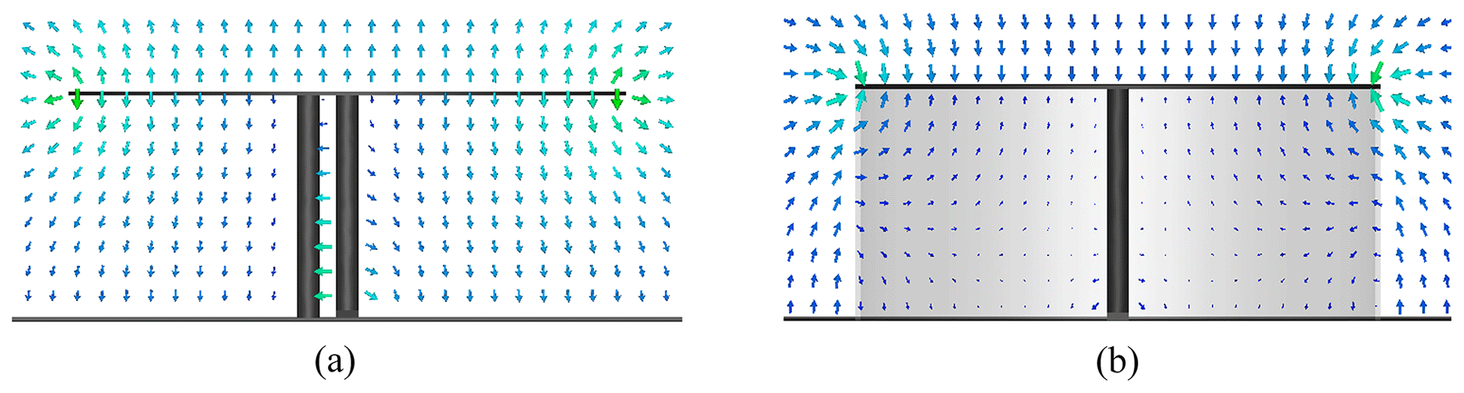
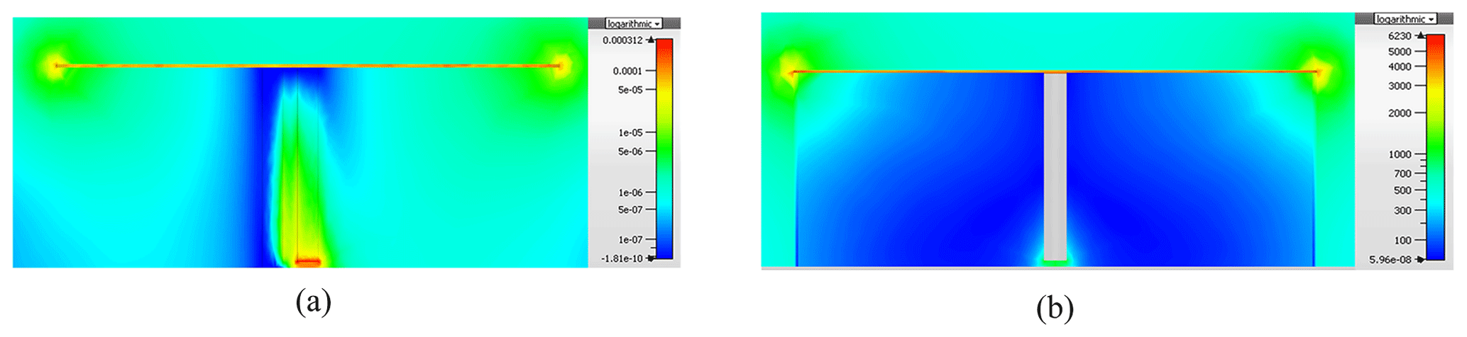
The internally stored electric energy (Q-energy) of a disk monopole antenna increases as compared to a monopole antenna without a top disk. Recently it was shown that the Q-energy can be significantly reduced and the bandwidth increased by shielding the disk monopole antenna using a thin magnetic material. In the present paper we consider the same structure to explain another method to increase the bandwidth by using a shield made of dispersive magnetic material. We apply the Kramers-Kronig transforms to derive physically correct real and imaginary parts of the dispersive magnetic material. We do not aim at a reduction of the internal energy but at a compensation of the electric by a magnetic stored energy for a wide frequency range. Disk monopole antennas with shells consisting of such dispersive permeability are finally numerically evaluated by means of a commercial frequency-domain field simulator.

Dates
1 Introduction

Because of their increasing importance electrically small antennas have often been discussed in the literature. An overview can be found in Hansen and Collin (2011). Generally the choice of an electrically small antenna narrows the antenna's bandwidth. Because of its inverse relationship to the stored energy the fractional bandwidth can be increased and consequently the quality factor (Q factor) can be reduced by minimizing the electric and the magnetic stored energy of the antenna. In a fundamental work, Chu (1948) showed that the lower bound of the Q-factor of an omnidirectional linear non-dispersive antenna is given by

(1) Q Chu η 1 ( k r ) 3

where k and r represent the wave number and the radius of the minimum sphere, respectively. In Eq. (1) the radiation efficiency η includes all of the losses.

Many techniques have been suggested and investigated for reducing the Q-factor of electrically small antennas. A few examples include but are not limited to the works by Hansen and Collin (2011), Yaghjian and Best (2005), Madsen et al. (2016), Best (2009), and Yaghjian and Stuart (2010). For low-frequency electromagnetic fields Stuart and Yaghjian (2010) introduced a high-permeability magnetic shell to eliminate the stored electric energy of a disk-loaded monopole antenna, resulting in a Q-factor nearby QChu.

The role of the Q-energy for an antenna containing dispersive media has been discussed in Yaghjian (2018). In that paper it was shown that the bound in Eq. (1) can be overcome by using tuning elements containing highly dispersive lossy material - however, the related increase of bandwidth was at the cost of a reduced efficiency.

In this paper we further investigate the aforementioned example of a disk-loaded monopole antenna (Stuart and Yaghjian2010) by shielding it with a dispersive magnetic material. However, we do not aim at a minimized stored energy. Instead we initially calculate frequency-wise the optimum permeability of the shielding material leading to a stored magnetic energy which equalizes the stored electric energy. Subsequently we calculate the related imaginary part of the permeability (i.e. the magnetic losses) by numerically applying the Kramers-Kronig (KK) transforms. Finally these results are inserted into a full-wave electromagnetic simulator to find the characteristics of the antenna.

The paper is organized as follows: We first derive an expression for the real part of the permeability of the dispersive shell leading to an equivalence of stored electric and magnetic energies. Next we apply the Kramers-Kronig transform to obtain the corresponding imaginary part of the permeability. We also check the consistency of the method, i.e., if the repeated application of the Kramers-Kronig transforms delivers the correct (initial) values of the real part of the permeability. Finally we numerically investigate the effect of shielding the disk monopole antenna by the designed magnetic dispersive material on the antenna's performance by applying a commercial frequency-domain solver.

2 Disk monopole antenna with a dispersive shell

Assume a disk monopole antenna as shown in Fig. 1 with negligible conductivity losses of the antenna structure. The antenna is driven by a coaxial cable where its center conductor works as the feed line. Both, the radius rc and the height h of the feed line are much smaller than the operating wavelength (Stuart and Yaghjian2010).

https://www.adv-radio-sci.net/17/65/2019/ars-17-65-2019-f01

Figure 1Cross sectional view of a disk monopole antenna (a) with a shorting post (SP) and (b) with a dispersive magnetic shield including the definitions of the different volumes va, vb, v0, and v. Due to the symmetry, only half of the cross section is shown for (b).

Download

To reduce the electric energy below the cap the antenna is often equipped with a shorting post (SP) as shown in Fig. 1a. Following the approach described by Stuart and Yaghjian (2010) we shield the unfolded disk monopole antenna by a magnetic material located symmetrically around the feed line (see Fig. 1a). Differently from Stuart and Yaghjian (2010) we choose a dispersive magnetic material for the shield. Figure 1b shows the geometry where due to the symmetry only half of the cross section is displayed.

https://www.adv-radio-sci.net/17/65/2019/ars-17-65-2019-f02

Figure 2Real (a) and imaginary (b) parts of the relative permeability of the dispersive shielding material for two values of A0. Geometry data (see Fig. 1): h=40, rb=50, rc=2.1, t=0.7, d=1 mm. (a) Comparison between the initial (original) values of the real part of the permeability μ calculated from Eq. (13) (solid curves) and the double Kramers-Kronig (DKK) transformed values (broken curves) calculated using Eqs. (15a) and (15b). (b) Imaginary part of the relative permeability μ′′ calculated by Eq. (15b) from the initial values of μ.

Download

We introduce a cylindrical coordinate system ρ,ϕ,z where the feed line is on the z-axis. A time-harmonic field with time-factor ejωt is assumed and omitted throughout the analysis. For the antenna structure in Fig. 1b it can be shown that the fundamental resonant mode is Transverse Magnetic (TMz) with an electric field E=Eρρ^+Ezz^ and a magnetic field H=Hϕφ^. Following the analysis and argumentation in Stuart and Yaghjian (2010) the Eρ-component is neglected. According to Ampères law the magnetic field is represented in terms of the current on the feed line as

(2) H ϕ ( ω , ρ ) = I ( ω ) 2 π ρ .

The electric field is found by applying Faraday's law to Eq. (2)

(3) C ( F ) E d s = - j ω F μ H d f E z ( ρ ) = - j ω μ I 2 π ln ρ r c .

The shield's permeability is described by μ(ω)=μ(ω)-jμ′′(ω) while the permittivity is supposed to be that one in vacuum ε=ε0. We aim at calculating those frequency-varying values μ(ω) leading to equivalent electric and magnetic stored energies for all frequencies in the desired frequency range. According to Yaghjian and Best (2005, Eq. 43) the complex input power of the antenna is related to the input impedance Zin(ω)=R0(ω)+jX0(ω) by

(4) P in ( ω ) = 1 2 I ( ω ) 2 Z in ( ω ) = P acc ( ω ) + j 2 ω ( W m ( ω ) - W e ( ω ) )

where Pacc is the time-averaged power accepted by the antenna and Wm, We are the stored magnetic and electric energies, respectively. For a linear homogeneous non-dispersive material the stored energies of the antenna can be written in terms of the frequency-domain fields (phasors) according to

(5)Wm(ω)=14RevB*Hdv(6)We(ω)=14RevD*Edv

where the asterisk (*) denotes the complex conjugation and where v is the total volume enclosing the antenna as shown in Fig. 1b.

Since the permeable shielding material is dispersive, Eq. (5) is no longer valid. The time-averaged energy in a dispersive material does not depend only on the instantaneous values of the material parameters (μ(ω) and ε(ω)) but also on their frequency derivatives (Landau and Lifshitz1960). Hence Eq. (5) must be rewritten for the volume vb according to

(7) W m ( ω ) | v b = 1 4 v b d ( ω μ ( ω ) ) d ω H ϕ 2 d v

while the total stored magnetic energy is estimated as

(8) W m ( ω ) = 1 4 d [ ω μ ( ω ) ] d ω v b H ϕ 2 d v + μ 0 v a + v 0 H ϕ 2 d v = I ( ω ) 2 4 d [ ω μ ( ω ) ] d ω 1 ( 2 π ) 2 v b 1 ρ 2 d v = L ̃ 1 + μ 0 1 ( 2 π ) 2 v a + v 0 1 ρ 2 d v = L ̃ 2 = I ( ω ) 2 4 d [ ω μ ( ω ) ] d ω L ̃ 1 + μ 0 L ̃ 2

where v0 represents an equivalent extension of the volume under the cap which is imaginarily extended by Δr (see Fig. 1b). This equivalent extension is due to the fringing fields at the rim of the cap. As shown in Chew and Kong (1980, Eq. 33) Δr can be estimated as

(9) Δ r 2 r b h π ln ( r b 2 h ) + 0.665 h r b + r b 2 1 2 - r b .

The total stored electric energy is calculated as

(10) W e ( ω ) = 1 4 v b ε 0 E z 2 d v + v a + v 0 ε 0 E z 2 d v = I ( ω ) 2 4 ω 2 μ 2 ( ω ) ε 0 ( 4 π ) 2 v b ln 2 ρ r c d v = C ̃ 1 + ω 2 μ 0 2 ε 0 ( 4 π ) 2 v a + v 0 ln 2 ( ρ r c d v = C ̃ 2 = I ( ω ) 2 4 ω 2 μ 2 ( ω ) C ̃ 1 + ω 2 μ 0 2 C ̃ 2 .

At resonance the total input reactance X0 is zero. Accordingly the magnetic and electric stored energies in Eq. (5) are equal, Wm(ω)=We(ω). Thus, from Eqs. (8) and (10) we have

(11) d [ ω μ ( ω ) ] d ω L ̃ 1 + μ 0 L ̃ 2 = ω 2 μ 2 ( ω ) C ̃ 1 + ω 2 μ 0 2 C ̃ 2 d μ ( ω ) d ω + 1 ω μ ( ω ) - C ̃ 1 L ̃ 1 ω μ 2 ( ω ) = ω μ 0 2 C ̃ 2 L ̃ 1 - 1 ω μ 0 L ̃ 2 L ̃ 1 .

Equation (11) represents a Riccati differential equation which generally can be difficult to solve. However, we follow Stuart and Yaghjian (2010) and assume that the stored energy is concentrated in the dispersive shell, i.e., μvbμ0(va+v0) (see Eqs. 8 and 10). Consequently we neglect the right-hand side in Eq. (11) and obtain the Bernoulli differential equation

(12) d μ ( ω ) d ω + 1 ω μ ( ω ) = C ̃ 1 L ̃ 1 ω μ 2 ( ω ) .

The solution of Eq. (12) can be easily obtained as

(13) μ ( ω ) = 1 - C ̃ 1 L ̃ 1 ω 2 + A 0 ω

where A0 is an arbitrary constant of dimension AmV.

https://www.adv-radio-sci.net/17/65/2019/ars-17-65-2019-f03

Figure 3Input impedance of the open disk monopole (no shielding) (green curves) and of the shielded disk monopole antenna (red curves). Geometry of the antenna: h=40, rb=50, rc=2.1, t=0.7, d=1 mm, A0=8.3×10⁻¹³s/Ω. Simulation using the CST© frequency-domain solver.

Download

https://www.adv-radio-sci.net/17/65/2019/ars-17-65-2019-f04

Figure 4Input return loss of the open disk monopole (no shielding) (blue curve) and of the shielded disk monopole antenna (red curve). The other data can be found in Fig. 3.

Download

https://www.adv-radio-sci.net/17/65/2019/ars-17-65-2019-f05

Figure 5Antenna gain of the open disk monopole (no shielding) (blue curve) and of the shielded disk monopole antenna (red curve). The other data can be found in Fig. 3.

Download

https://www.adv-radio-sci.net/17/65/2019/ars-17-65-2019-f06

Figure 6Electric field distribution (a) of the open disk monopole (with shorting post) at f0=437 MHz and (b) of the shielded disk monopole at f=200 MHz. The other data can be found in Fig. 3.

Download

https://www.adv-radio-sci.net/17/65/2019/ars-17-65-2019-f07

Figure 7Electric energy density (a) of the open disk monopole (with shorting post) at f0=437 MHz and (b) of the shielded disk monopole at f=200 MHz. The other data can be found in Fig. 3.

Download

3 Kramers-Kronig transformation

In a magnetically dispersive material the magnetic flux density B(t) is related to the magnetic field intensity H(t) by the causal convolution

(14) B ( t ) = 0 t μ ( τ ) H ( t - τ ) d τ .

Equivalently, in the frequency domain the real and imaginary components of μ have to satisfy the Kramers-Kronig transforms (Kramers1927), (Kronig1926) according to

(15a)μ(ω)=1+2π0ω^μ′′(ω^)-ωμ′′(ω)ω^2-ω2dω^(15b)μ′′(ω)=-2ωπ0μ(ω^)-μ(ω)ω^2-ω2dω^.

First we calculate μ(ω) from Eq. (12) by choosing the constant A0 such that we obtain a positive permeability. Exemplarily, we consider the disk monopole antenna of Fig. 1 with the dimensions h=40, rb=50, rc=2.1, t=0.7, d=1 mm. As shown in Fig. 2a μ(ω) is evaluated according to Eq. (12) as a function of the angular frequency for different values of A0. Next, we apply Eq. (15b) to numerically calculate the corresponding μ′′(ω) as shown in Fig. 2b. For the numerical procedure (splitting the integration ranges, spline-based extrapolation) we have used the same technique as we developed and described in Bakry and Klinkenbusch (2018). To check the consistency of the method we performed an additional Kramers-Kronig transform according to Eq. (15a) on the data shown in Fig. 2b. The results (dotted curves in Fig. 2a) are in good agreement to the initial values of μ(ω) (solid curves).

4 Numerical results

Both types of the disk monopole antennas in Fig. 1a with shorting post and Fig. 1b with a dispersive permeable shield were simulated using a commercial field solver (CST©, frequency-domain solver). The characteristic impedance of the feed line is 50 Ω. The fundamental resonance frequency for the non-shielded antenna has been found to be f0=437 MHz. Figures 3 and 4 show the input impedance and the return loss, respectively, of both antenna types, each as a function of the frequency. It is obvious that the antenna Q is much higher for the non-shielded antenna and that the resonance frequency moves to a higher frequency. Overall, it is observed from Figs. 3 and 4 that the bandwidth can be drastically increased by using dispersive permeable material. At low frequencies the input resistance approaches the feed line resistance while the return loss is relatively constant and low. However, because of the high losses of the dispersive shielding material it is expected and shown in Fig. 5 that the gain for the shielded antenna is drastically reduced.

As proven in Stuart and Yaghjian (2010) the shielding of the antenna by a non-dispersive high-permeability shell leads to a reduced electric field in the shielded domain. As shown in Fig. 6 this fact can also be proven for a dispersive shell with high permeability. Correspondingly, Fig. 7 finally represents the reduction of the stored electric energy within the shielded domain.

5 Conclusions

We have introduced a systematic method showing that the numerical evaluation of the Kramers-Kronig transformations can be used to design wide-band antennas consisting of dispersive material. In the future the method will also be applied to other antenna geometries and to a material with a negative value of the real part of the permeability and/or permittivity (metamaterial) to eventually avoid the high dispersion losses and the corresponding reduced gain.

Data availability

The data are available from the authors upon request.

Author contributions

The theoretical work was done by LK and MB. The numerical evaluation was performend by MB.

Competing interests

The authors declare that they have no conflict of interest.

Special issue statement

This article is part of the special issue “Kleinheubacher Berichte 2018”. It is a result of the Kleinheubacher Tagung 2018, Miltenberg, Germany, 24–26 September 2018.

Financial support

This research has been supported by the Deutscher Akademischer Austauschdienst (DAAD) and the Egyptian Ministry of Higher Education and Scientific Research within the GERLS program.

Review statement

This paper was edited by Thomas Eibert and reviewed by Hans-Jürgen Steiner and three anonymous referees.

References

Bakry, M. and Klinkenbusch, L.: Using The Kramers-Kronig Transforms To Retrieve The Conductivity From The Effective Complex Permittivity, Adv. Radio Sci., 16, 23–28, https://doi.org/10.5194/ars-16-23-2018, 2018. a

Best, S. R.: A Low Q Electrically Small Magnetic (TE Mode) Dipole, IEEE Antenn. Wirel. Pr., 8, 572–575, 2009. a

Chew, W. C. and Kong, J. A.: Effects of Fringing Fields on the Capacitance of Circular Microstrip Disk, IEEE T. Microw. Theory, 28, 98–104, 1980. a

Chu, L. J.: Physical Limitations of Omni-Directional Antennas, J. Appl. Phys., 19, 1163–1175, 1948.  a

Hansen, R. C. and Collin, R. E.: Small Antenna Handbook, Wiley and IEEE Press, 2011. a, b

Kramers, H. A.: La diffusion de la lumiere par les atomes (1927), in: Collected Scientific Papers by H. A. Kramers, North-Holland Pub. Co., 1956. a

Kronig, R. de L.: On the Theory of Dispersion of X-rays, J. Opt. Soc. Am., 12, 547–557, 1926. a

Landau, L. D. and Lifshitz, E. M.: Electrodynamics of Continuous Media (2nd impression), Oxford, Pergamon Press, 253–256, 1963. a

Madsen, K. N., Zhou, Y., and Sievenpiper, D. F.: A Simplified Low-Q Electrically Small Magnetic Dipole Antenna, IEEE Antenn. Wirel. Pr., 15, 1975–1978, 2016. a

Stuart, H. R. and Yaghjian, A. D.: Approaching the Lower Bounds on Q for Electrically Small Electric-Dipole Antennas Using High Permeability Shells, IEEE T. Antenn. Propag., 58, 3865–3872, 2010. a, b, c, d, e, f, g, h

Yaghjian, A. D.: Overcoming The Chu Lower Bound on Antenna Q with highly dispersive lossy material, IET Microwaves, Antenn. Propag., 12, 459–466, 2018. a

Yaghjian, A. D. and Best, S. R.: Impedance, Bandwidth, and Q of Antennas, IEEE T. Antenn. Propag., 53, 1298–324, 2005. a, b

Yaghjian, A. D. and Stuart, H. R.: Lower Bounds on the Q of Electrically Small Dipole Antennas, IEEE T. Antenn. Propag., 58, 3114–3121, 2010. a

Download
Short summary
In this paper we explain a novel method to increase the bandwidth of a top-loaded monopole antenna by using a shield made of dispersive magnetic material. We apply the Kramers-Kronig transforms to derive physically correct real and imaginary parts of the dispersive magnetic material. We aim at a compensation of the electric by a magnetic stored energy for a wide frequency range. Independent numerical solutions using the commercial field solver CST support the results of our investiagation.