 | 19 Sep 2019
Multilayered Transmission Lines on Quasi-planar Substrates With Anisotropic Medium
Achim Dreher
This paper exhibits the extension of the discrete mode matching (DMM) method to analyze conformal structures with anisotropy. It represents a simple formalism as a basis to analyze multilayered structures with quasi-planar anisotropic dielectric layers. The dyadic Green's function is then calculated using a full-wave equivalent circuit (FWEC) of the structure, where each layer is represented with the hybrid block consisting of the tangential field components. The application is demonstrated by computing propagation constants for partially filled quasi-planar waveguides and microstrip lines with isotropic, uniaxial and biaxial anisotropic dielectrics.
- Article
(2680 KB) - Full-text XML
- BibTeX
- EndNote


Microstrip structures are very widely used in antennas and microwave devices for navigation and communication systems in transport, aeronautics and space. Often there is need to integrate them into the surface of aircraft, satellites and vehicles, which leads to the structures to be conformal (Yinusa, 2018). New lightweight materials (e.g. CFK) are being used more frequently in exhibiting multilayers with anisotropic behavior. Since the substrate material strongly affects the properties of the structures, the microwave circuit elements need to be modelled very precisely and fast numerical procedures are required to predict their characteristics.
In the literature, we can find the work done for analyzing waveguides with arbitrary cross-section using different methods. For example, Horikis (2013) used the finite difference technique, Yee and Audeh (1965) used the point matching technique, She (1989) used the iterated moment method and Yang and Pregla (1996) used the method of lines (MoL) to analyze conformal structures. Here the focus is on the full-wave analysis method known as discrete mode matching (DMM) method, which was earlier successfully used to analyze microwave structures with high accuracy. For example, Kamra and Dreher (2018a) explained the DMM formulation to analyze transmission lines with multiple strips, Kamra and Dreher (2019) dealt with circular and non-circular dielectric layers with uniaxial anisotropy. The conformal transmission lines with quasi-planar substrate were also examined using this method but with isotropic media (Dreher and Ioffe, 2000).
The present contribution extends the efficient numerical method, i.e. DMM, to analyze conformal structures with anisotropic materials. This method uses the exact eigenvalues of the waveguide modes, which are dependent on the lateral boundary conditions. It requires only 1-D discretization along the horizontal tangential direction of the interfaces for the analysis of multilayered transmission line structures as the structure is assumed infinite in the propagation direction. In the direction perpendicular to the interfaces, the analytical solution is taken. Here, each layer is defined by a hybrid matrix which relates the tangential field components at its interfaces. The shape of the interfaces can be defined by the suitable equation, from which the slope at each discretization point can be calculated. Consequently, the field components are determined for each sampling point in the interfaces with varying slope. Then the dyadic Green’s function (or system equation) is derived using a full-wave equivalent circuit (FWEC) in the space domain. The application is demonstrated by computing propagation constants for quasi-planar waveguide and stripline having uniaxial or biaxial anisotropic dielectric layers and the results are validated with those obtained with commercial software, ANSYS HFSS.
2.1 Field equations
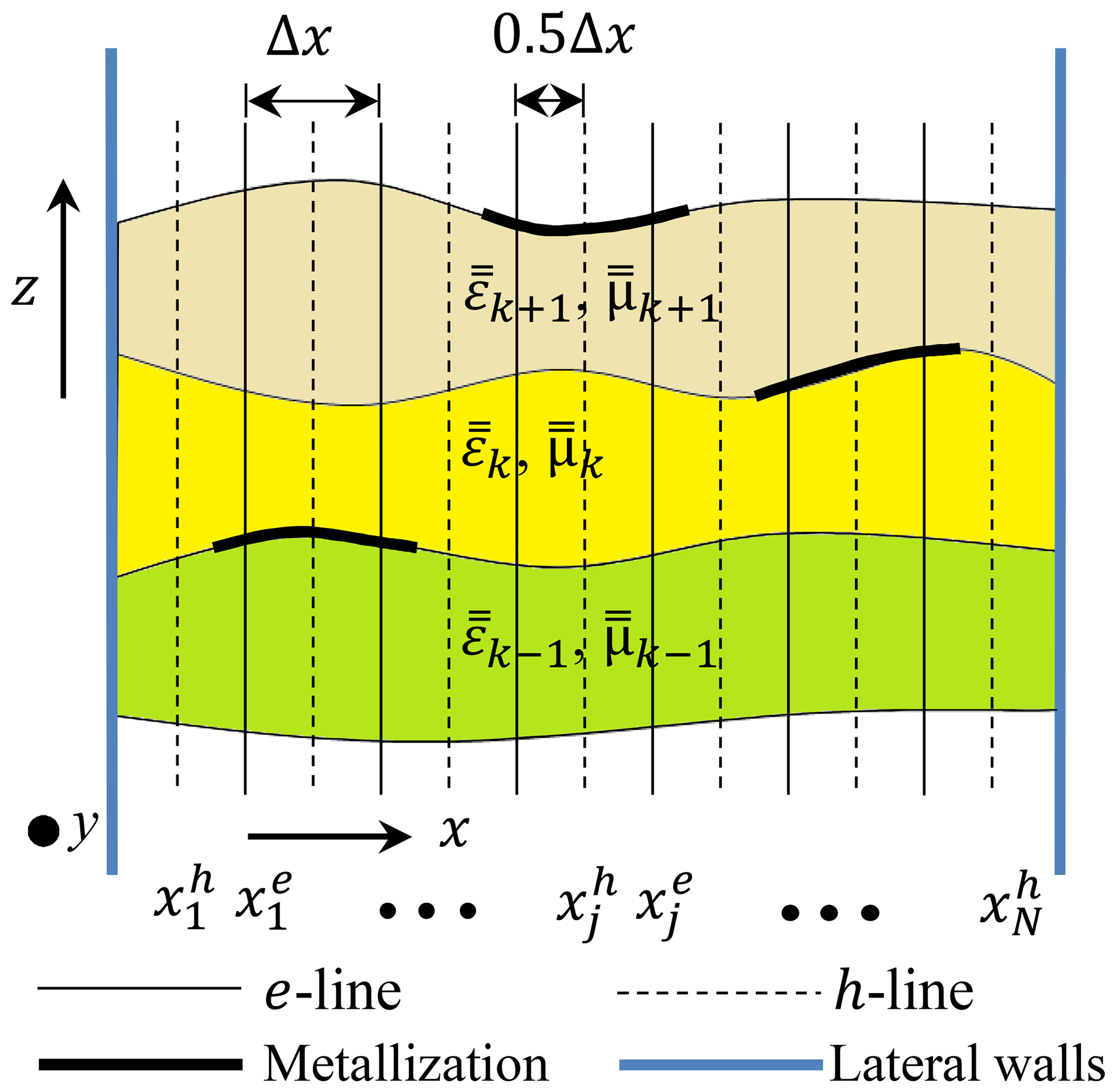
We depict the general cross-section of the microwave structure with arbitrarily shaped dielectric layers in Fig. 1. Here we consider several microstrip lines in the interfaces of the dielectric layers. For the present analysis, we take the stratification of the structure in z-direction and the wave propagation (exp (−jkyy)) in y-direction. The permittivity () and permeability () tensor of the dielectric layer can be written with
It is mentioned by Krowne (1984) that we should begin our analysis by taking any of the two independent field components. Hence, we start our analysis with two scalar fields Ey and Hy. From the source-free Maxwell's equations normalized by the free-space wave number k0, the relation between the field components can be written as
where is replaced by with . After applying the Fourier transform, we obtain two coupled second-order differential equations
where
From Eqs. (5) and (6), we can write that TEy and TMy modes cannot exist for the biaxial case. On elimination of the other coupled field component or from Eqs. (5) or (6) respectively, we get a fourth-order differential equation
with or . The four analytical solutions () can be computed from Eq. (8) with
where the field solution is with . When we take , then the solution can be written as
From Eq. (6), we can write
Therefore combining Eqs. (10) and (11), we get
where and .
For the uniaxial case with optical axis in y-direction, variables b and d become zero in Eqs. (5) and (6) respectively. Therefore, we get two uncoupled differential equations which can be solved as explained in Kamra and Dreher (2018b). Similarly, the independent field components should be Ex, Hx and Ez, Hz for the optical axis in x- and z-direction respectively. The isotropic case can be solved with either pair of the independent field components.
2.2 Discrete mode matching method
We assume the structure to be infinite in the propagation direction, so we need just 1-D discretization along x for the analysis of multilayered microstrip line as shown in Fig. 1. We sample the field components at N equidistant points xj between the lateral walls. In the figure, e-lines show the position of Ey and h-lines show the position of Hy field component. The modal expansion of field components having N modes discretized by N samples is given by
Here T is the transformation matrix (Fourier series elements) using the exact eigensolutions τ(kxixj) of the wave equation which are dependent on the lateral boundary conditions and i denotes the index for modes while j denotes the index of the samples.
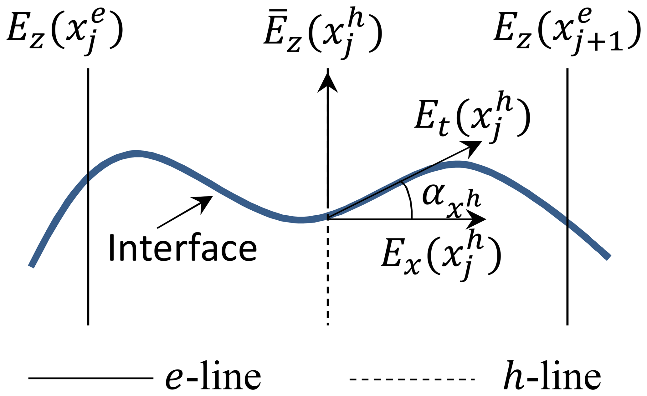
We assume that for an arbitrary layer k the cross-section is constant in the y-direction, therefore Ey and Hy are tangential to the interfaces along the whole x-direction. The quasi-planar nature of the layers at the interfaces is in x-direction, therefore the other tangential fields become Et and Ht, and are represented as
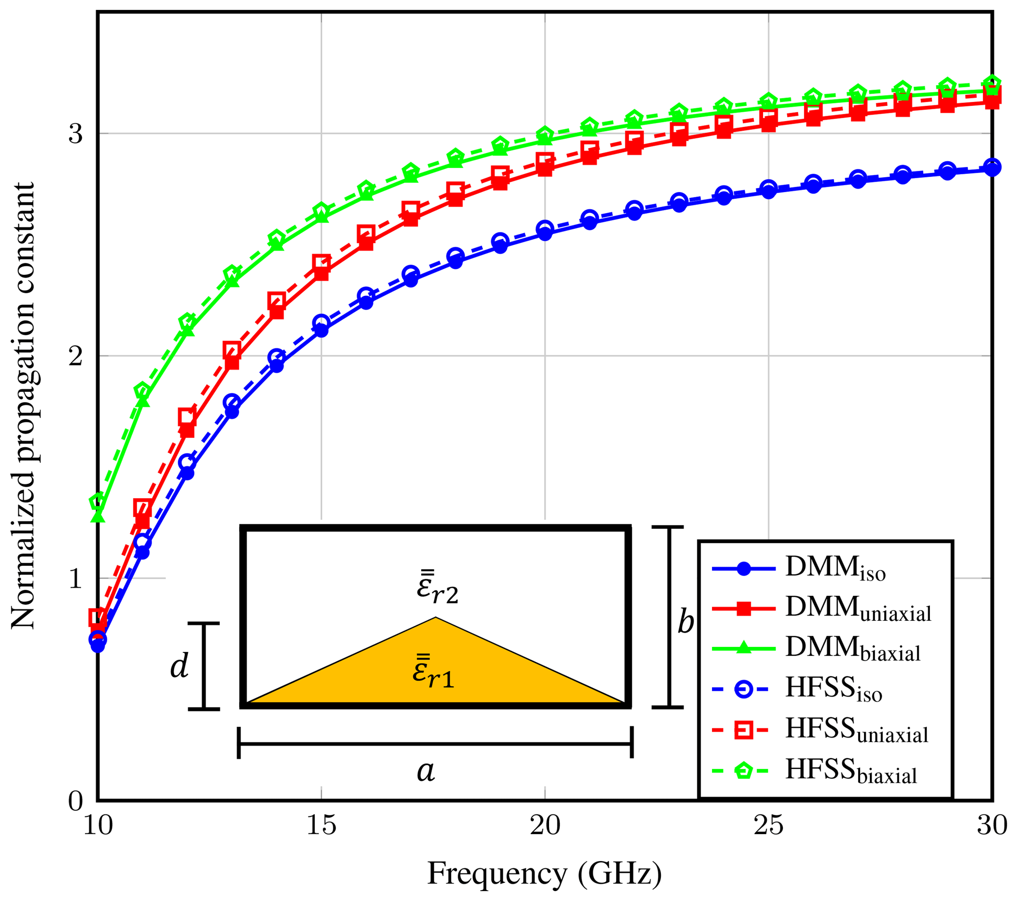
Figure 3Dispersion curve for the partially filled waveguide with triangular dielectric layer.
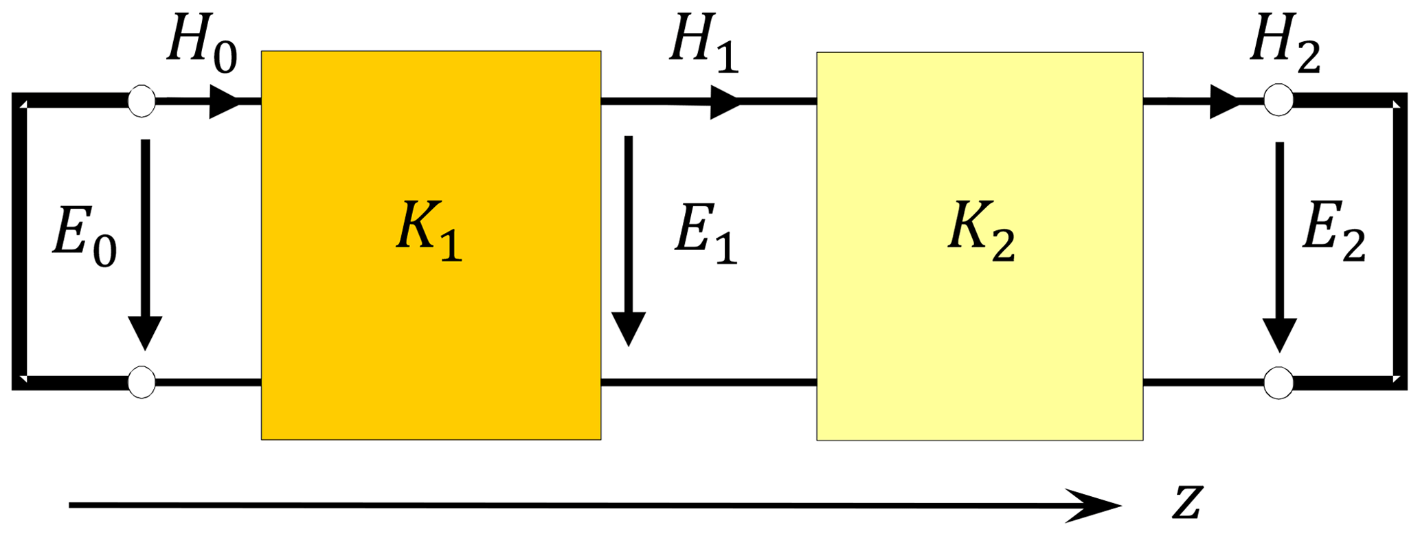
Figure 2 clarifies the tangential field component calculation and here represents the inclination angle at the interface with the x-axis. From Eqs. (3)–(4), we can say that for 1-D discretization Ez, Ey and Hx (or Hz, Hy and Ex) components are sampled at the same position. To determine Et, we must calculate Ex and Ez at the same point. Therefore, we use in Eq. (14a) which is the mean of the adjacent sampled values of Ez. Similarly, is calculated from the mean of the adjacent sampled values of Hz.
We calculate the hybrid matrix of the layer in a similar way as explained in (Kamra and Dreher, 2018b) but here we consider discretization also alongwith. And for quasi-planar structures we deal with the equations in space domain (Eqs. 3–4) rather than in spectral domain. We obtain the discretized field relations for layer k as
on taking the notations of the fields and coefficients in the vector form as
After eliminating the unknown coefficient vector F, it results in
The hybrid matrix (Kk) for layer k can be represented as
The system equation can be formed on using the network analysis technique and the continuity equations on the interfaces to match the fields. Then the boundary conditions which state that the tangential electric field components must vanish on the metallizations and the electric currents outside that region must be applied. We obtain the reduced system equation as
which can be solved as an indirect eigenvalue problem (det(Gred)=0 or det(Lred)=0) to find the propagation constants for the transmission lines. Here denotes the dyadic Green's function and Lred is equivalent to L in waveguides, as there are no currents on the interfaces.
3.1 Waveguides
First, we have applied the DMM formulation to analyze partially filled waveguide whose inner layer is taken to be in triangular shape. The schematic is shown in the inset of Fig. 3. The data used for the analysis are: b=6.35 mm, a=2b, d=0.5b, or (9.4, 9.4, 11.6) or (9.4, 13, 11.6), εr2=1. Figure 4 gives the FWEC obtained from the structure where K1 and K2 represent the hybrid matrices for the layer 1 and 2 respectively. From the circuit, we can deduce the system equation as
Figure 3 shows the dispersion curves, normalized by k0, obtained after solving the eigenvalue problem. For the present computation, we have analyzed only half of the structure due to symmetry and have used 17 e-lines to discretize it. The results agree well with the results obtained from ANSYS HFSS. Then, Fig. 5 demonstrates six higher order modes computed for the biaxial case of the waveguide shown in the inset of Fig. 3. The figure validates the DMM results with the commercial software.
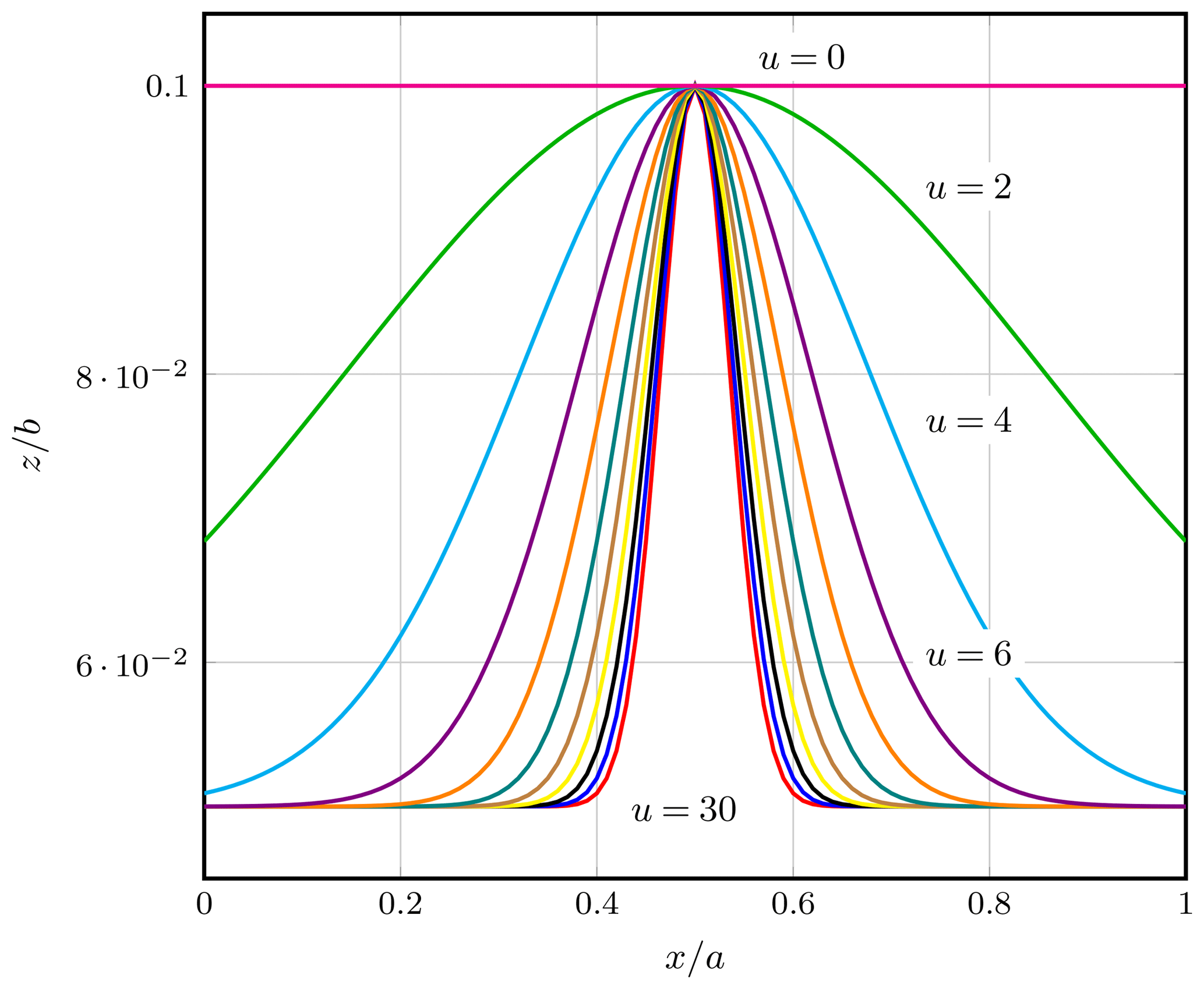
Then, we have changed the inner interface within the waveguide with the function
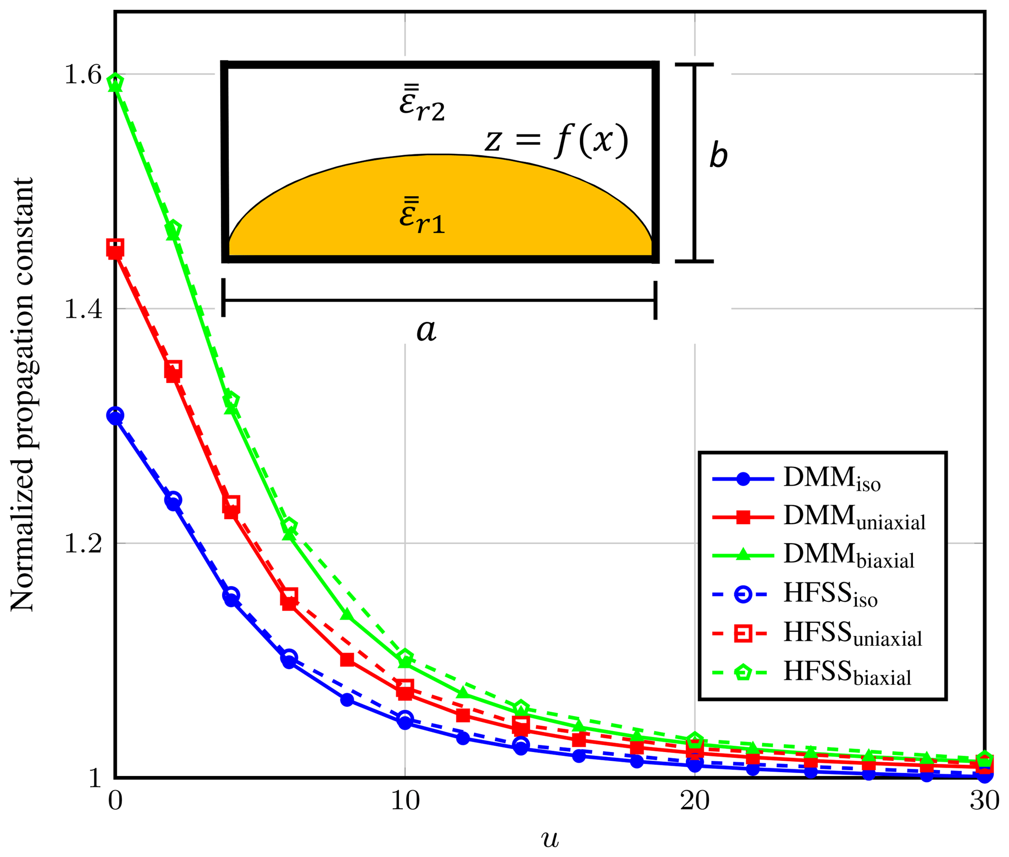
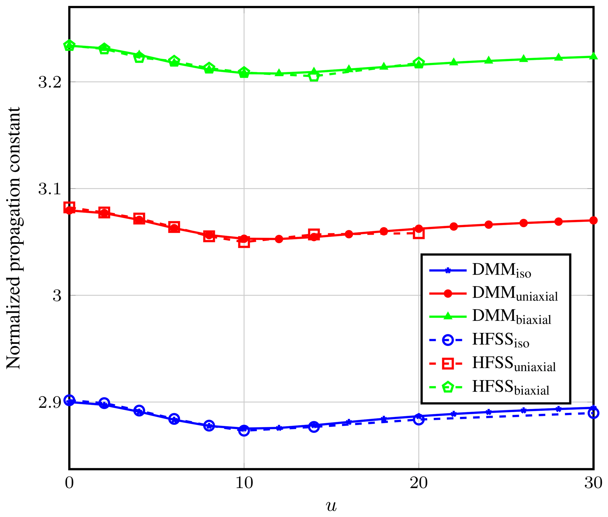
and have analyzed the structure with the following parameters: b=7.5 mm, a=2b, or (8.875, 8.875, 15) or (8.875, 10, 15), εr2=1. The shape of the interface varies with the value of u as shown in Fig. 6. Figure 7 gives the computed values of the normalized propagation constant with varying u. We have used 22 e-lines for discretizing half of the structure. The figure compares the DMM results for the isotropic, uniaxial and biaxial anisotropic medium with the results from the HFSS. We have computed the results at 30 GHz frequency.

3.2 Microstrip line
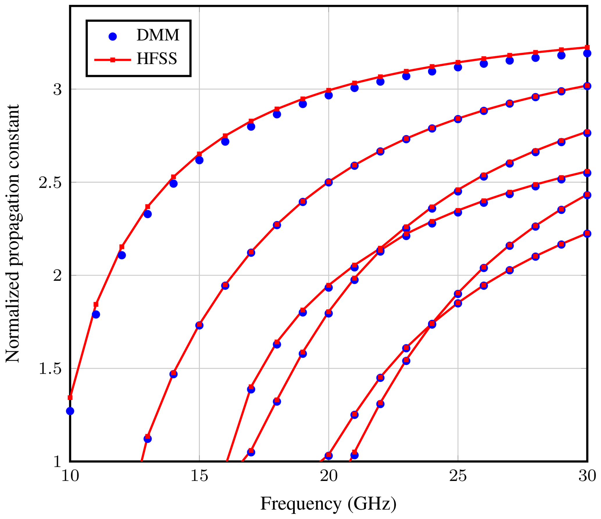
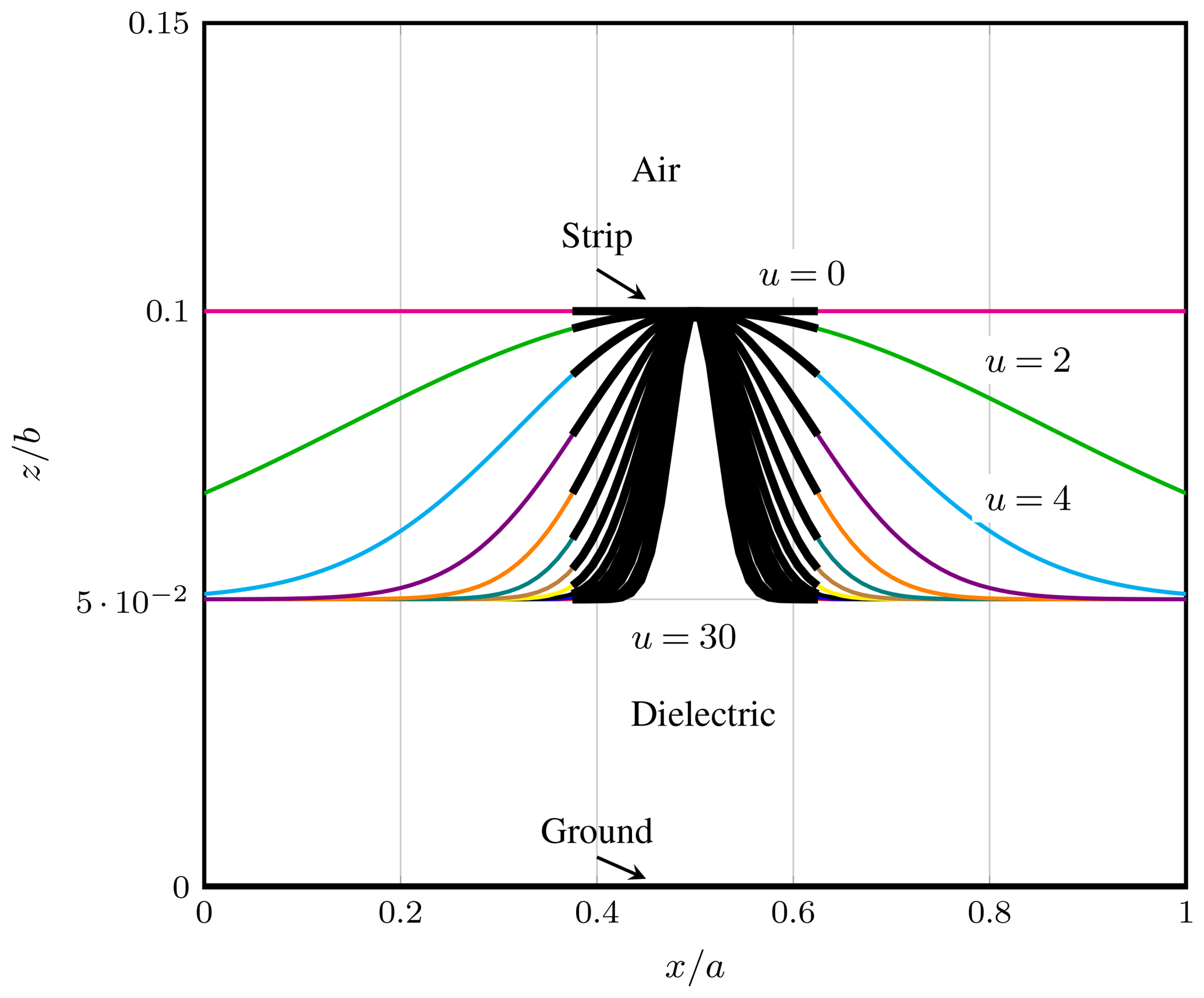
Next, we have analyzed a microstrip line where the strip is placed on the inner interface of the structure shown in Fig. 7. The inner layers of the structure are taken with relative permittivity or (8.875, 8.875, 10) or (8.875, 9, 11) and εr2=1. The cross section of the structure is with b=7.5 mm and a=2b, and has strip width w=0.25a. Figure 8 clearly shows the variation of the strip with the interface. We obtain the FWEC of the quasi-planar stripline as depicted in Fig. 9. The system equation for the two layer microstrip line takes the form as
where J1 gives the currents on the strip (Fig. 9).
Figure 10 shows the computed results at 30 GHz frequency with DMM and HFSS. For DMM computation, we have used 12 e-lines on half of the strip for isotropic and uniaxial case and 6 e-lines for biaxial case. In HFSS, the consumed time span for the analysis at each u-point varied between 26 s to 1 h, while with DMM formulation it was between 10 to 12 s. We have used the same number of segments for all values of u in HFSS and also the same number of discretization lines in DMM to clearly interpret the curvy interface. However, HFSS needs more meshes and computation time to smoothly analyze the interface with higher value of u. While for DMM, computation time doesn't vary much for different values of u. With the same number of discretization lines, it depends only on how much time is needed to calculate the roots of the eigenvalue problem.
The efficient full-wave analysis method (DMM) has been presented to analyze quasi-planar transmission lines with anisotropic stratified media. The method can also easily deal with multilayered structures with metallizations in different interfaces. Both waveguides and stripline structures were analyzed with good agreement with the commercial software. The method can also be extended for the analysis of microstrip patch antenna on quasi-planar anisotropic substrate with 2-D discretization.
There are no underlying research data for the presented work. All results can be reproduced with the equations and parameters given directly in the paper.
The authors declare that they have no conflict of interest.
This article is part of the special issue “Kleinheubacher Berichte 2018”. It is a result of the Kleinheubacher Tagung 2018, Miltenberg, Germany, 24–26 September 2018.
This research has been supported by the DLR/DAAD Research Fellowship (grant no. 57186656).
The article processing charges for this open-access
publication were covered by a Research
Centre of the Helmholtz Association.
This paper was edited by Thomas Eibert and reviewed by three anonymous referees.
Dreher, A. and Ioffe, A.: Analysis of microstrip lines in multilayer structures of arbitrarily varying thickness, IEEE Microw. Guided W., 10, 52–54, 2000. a
Horikis, T. P.: Dielectric waveguides of arbitrary cross sectional shape, Appl. Math. Model., 37, 508 –5091, 2013. a
Kamra, V. and Dreher, A.: Efficient Analysis of Multiple Microstrip Transmission Lines With Anisotropic Substrates, IEEE Microw. Wirel. Co., 28, 636–638, 2018a. a
Kamra, V. and Dreher, A.: Full-wave equivalent circuit for the analysis of multilayered microwave structures with anisotropic layers, Electron. Lett., 54, 153–155, 2018b. a, b
Kamra, V. and Dreher, A.: Analysis of Circular and Noncircular Waveguides and Striplines With Multilayered Uniaxial Anisotropic Medium, IEEE T. Microw. Theory, 67, 584–591, 2019. a
Krowne, C.: Green's function in the spectral domain for biaxial and uniaxial anisotropic planar dielectric structures, IEEE T. Antenn. Propag., 32, 1273–1281, 1984. a
She, S. X.: Iterated-moment method for the analysis of optical waveguides of arbitrary cross section, J. Opt. Soc. Am. A, 6, 1031–1037, 1989. a
Yang, W. D. and Pregla, R.: The method of lines for analysis of integrated optical waveguide structures with arbitrary curved interfaces, J. Lightwave Technol., 14, 879–884, 1996. a
Yee, H. Y. and Audeh, N. F.: Uniform Waveguides with Arbitrary Cross-Section Considered by the Point-Matching Method, IEEE T. Microw. Theory, 13, 847–851, 1965. a
Yinusa, K. A.: A Dual-Band Conformal Antenna for GNSS Applications in Small Cylindrical Structures, IEEE Antenn. Wirel. Pr., 17, 1056–1059, 2018. a