 | 10 Dec 2020
Transparent boundary condition for the calculation of eigenmodes in transversely infinite waveguides
Mikhail Patrushev
Wolfgang Ackermann
Thomas Weiland
Waveguides play one of the key figures in today's electronics and optics for signal transmission. Corresponding simulations of electromagnetic wave transportation along these waveguides are accomplished by discretization methods such as the Finite Integration Technique (FIT) or the Finite Element Method (FEM). For longitudinally homogeneous and transversely unbounded waveguides these simulations can be approximated by closed boundaries. However, this distorts the original physical model and unnecessarily increases the size of the computational domain size. In this article we present a boundary condition for transversely open waveguides based on the Kirchhoff integral which has been implemented within the framework of FIT. The presented solution is compared with selected conventional methods in terms of computational effort and memory consumption.
- Article
(652 KB) - Full-text XML
-
Supplement
(484 KB) - BibTeX
- EndNote


In order to quantify electromagnetic wave propagation in longitudinally homogeneous waveguides, simulations are performed on a two-dimensional domain. Transversely unbounded waveguides such as the microstrip-line displayed in Fig. 1 or an on-chip open waveguide are often physically not enclosed by shields. For numerical simulations a specifically tailored boundary condition has to be considered.
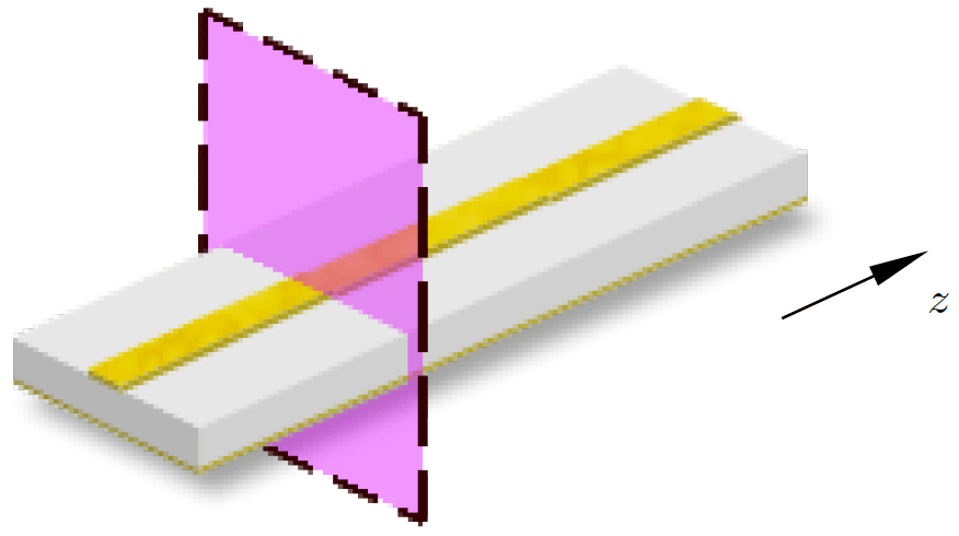
Figure 1Two-dimensional cross section in a reference plane used to calculate the modal fields on a transversely open microstrip line.
The two-dimensional problem of transversely unbounded waveguide can be calculated in terms of an eigenvalue problem. The required calculation is performed on a computational domain that consists in the considered case of a face and corresponding boundary conditions, by which the solution is defined. In contrary to closed waveguides, numerically efficient and physically correct representations of transversely open boundary conditions are still subject to research.
Simulations of the wave propagation along a three-dimensional, longitudinally homogeneous waveguides can be reduced to a two-dimensional formulation using the following ansatz:
with being the phasor of the electric field strength and being the propagation constant of a corresponding mode along the propagation direction z. On account of the underlying frequency-domain formulation, a time harmonic dependency of electromagnetic field is assumed. Inserting Eq. (1) in Maxwell's equations, an eigenvalue problem can be formulated, where the eigenvectors represent the phasors of the electric field strength in the transverse plane (also known as waveguide modes) and the eigenvalues describe the propagation constants for each individual mode. Each solution for these modes in transversely unbounded and longitudinally homogeneous waveguides can be approximated using closed boundary conditions.
2.1 Closed boundary conditions
Hollow waveguides with good electric conductive materials can be simplistically simulated using Perfect Electric Conductor (PEC) instead of the conductive material. In this case, an efficient implementation can use this boundary condition to represent the conducting material.
A Perfect Magnetic Conductor (PMC) can also be used to formulate a closed boundary. Dependent on the specific application, PMC or PEC also handles a suitable symmetry condition. With PMC or PEC boundary conditions, the solution contains propagating, evanescent or even complex modes, which appear as complex conjugate pairs.
If a transversely unbounded waveguide is artificially truncated with a PEC or PMC boundary condition, the resulting solution will be distorted, since either the tangential or the normal electric or magnetic field components will be missing. Furthermore, in transversely inhomogeneous waveguides, complex modes have to be considered (Strube and Arndt, 1985; Monsoriu et al., 2003; Clarricoats and Slinn, 1965). However, in case of a longitudinally homogeneous open waveguide complex eigenmodes are only present at very specific conditions (Jabłoński, 1994). Furthermore, it is also important that choosing between PEC or PMC requires an a priori knowledge of the field distribution of a specific mode. Thus, for TEM or Quasi-TEM modes the PMC might generally be suited better than the PEC boundary condition, since the PEC boundary condition itself introduces an additional conductor. In order to obtain an accurate solution, closed boundary conditions must be set further away from the original waveguide which naturally is accompanied by an increase of the computational cost due to the enlarged problem size.
2.2 Absorbing boundary conditions
Transversely open waveguide problems can also be addressed using absorbing boundary conditions like perfectly matched layers (PML) (Bérenger, 1994). There are different possibilities to implement PML (Roden and Gedney, 2000; Johnson, 2010) but independent of the formulation the underlying idea is not changed. The PML implements a boundary condition that contains one or multiple layers of nonphysical materials, that absorb the energy of incidenting electromagnetic wave. If PML is used as a transverse boundary condition for the case of longitudinally homogeneous waveguides, the propagation direction of the wave is directed parallel to the boundary. Hence, the assumed conditions for a PML boundary to function properly are not met. Additionally, a PML introduces nonphysical modes (Talukder, 2009; Rogier and De Zutter, 2001) that unfortunately distorts the physical solution spectrum. However, these modes can be identified (Bandlow et al., 2010). Furthermore, if the PML is enclosed by PEC or PMC, similar modes as described in Sect. 2.1 can arise.
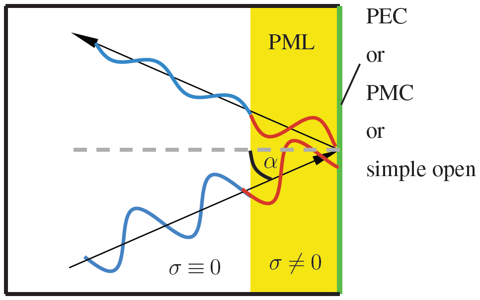
Figure 2The energy of an incoming wave traveling towards the boundary at the angle α is partially absorbed within the PML region. The PML layer is terminated by a closed boundary condition such as PEC or PMC or by a simple open condition.
The core idea for the realization of a physically correct transversely open boundary condition within the framework of FIT resides in (i) the evaluation of the field in the exterior domain and in (ii) its implication on the location of the boundary of the computational domain. In the presented approach, the electromagnetic field is evaluated using the Kirchhoff Integral (Jackson, 1998). Contrary to specifically available closed or absorbing boundary conditions, this approach defines a generally available open boundary condition. After a short survey of the fundamentals of Kirchhoff Integral as well as the basic principles of FIT, the combination of both will be used to formulate an open boundary condition.
3.1 Fundamentals of the Kirchhoff integral
In Fig. 3, a region R1, containing all the sources that are enclosed by a surface S1 and another surface S2 is considered. Hence, the region R2 is a source-free and homogeneous domain. Electromagnetic fields in region R2 generated by the sources in region R1 can be efficiently described by corresponding field components on the surface S1 (Jackson, 1998).
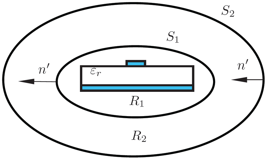
Figure 3Sources in the region R1 enclosed by the surface S1. An additional surface S2 is considered here, but will be moved to infinity afterwards for technical reasons.
Using the electric and magnetic field values on the surfaces S1 and S2, the electric or magnetic field strength in the region R2 can be evaluated. By expressing the magnetic field strength through the electric field strength , the calculation of the required fields inside the region R2 can be conducted using the surface integral
with n′ being the normal vector on the respective surfaces directed towards the region R2 and G(r) being the three-dimensional Green's Function for the Helmholtz equation (Jackson, 1998). By placing the surface S2 infinitely far away from S1, the surface integral (Eq. 2) has to be evaluated only along S1, as specified in Jackson (1998).
The required integration over the entire two-dimensional surface can be carried out partially on account of the a priori knowledge given in Eq. (1). As a result, a one-dimensional integral over a closed contour in the transverse plane of the investigated waveguide remains and can be summarized as
where , r) is the two-dimensional Green's function that additionally depends on the propagation constant due to the integration along the longitudinal coordinate. In the presented method, the open boundary problem is transferred into a nonlinear eigenvalue problem with being the desired eigenvalue. Hence, the linear eigenvalue problem in case of PMC or PEC boundary condition becomes nonlinear for the specified open boundary condition due to the two-dimensional Green's function being dependent on the eigenvalue.
3.2 Finite integration technique
The volume discretization method FIT (Weiland, 1977), Weiland (2017) is applicable for calculations in the frequency as well as in the time domain. It allocates electric and magnetic voltages and fluxes on a primal and a dual mesh. These field quantities are defined in FIT as integrals as follows1
Voltages and fluxes are allocated on mesh edges and faces, respectively, and are stored as algebraic vectors of dimension 3Np.
with Np being the number of mesh nodes. Material settings are expressed as material matrices, thus the corresponding material relations can be expressed as follows:
The required curl, divergence and gradient operators are defined on the primal and dual mesh as band matrices C, , S, , G, , respectively, with following properties
where the operators marked with a tilde are defined on the dual mesh. Assuming harmonic time dependence as before and substituting magnetic quantities by electrical quantities, a three-dimensional wave equation in the frequency domain can be formulated in form of the standard eigenvalue problem
where ω represents the angular frequency. The specified system matrix is sparse and unsymmetrical, but can be symmetrized. The three-dimensional problem (Eq. 6) can be reduced to two dimensions and formulated in a way such that becomes the eigenvalue (Weiland, 1977; Schmitt, 1994). As a result, the two-dimensional eigenvalue problem
can be derived. The system matrix A is sparse and unsymmetrical and can generally not be symmetrized.
3.3 Kirchhoff integral used as an open boundary condition for FIT
Consider the two-dimensional rectangular mesh specified in Fig. 4. The presented Kirchhoff Integral boundary (KIR) evaluates the electric field at the boundary Bc of the computational domain via Eq. (3). For this evaluation, the electric field values on the reference boundary Br are used. In order to study the influence of the singularity in the Green's function on the modeling accuracy, a variable spatial distance between Bc and Br is introduced. Since Eq. (3) depends on , the two-dimensional eigenvalue problem with KIR as a boundary condition becomes nonlinear. FIT 2D eigenvalue matrix (Eq. 7) becomes denser and non symmetrizable if KIR is used as a boundary condition.
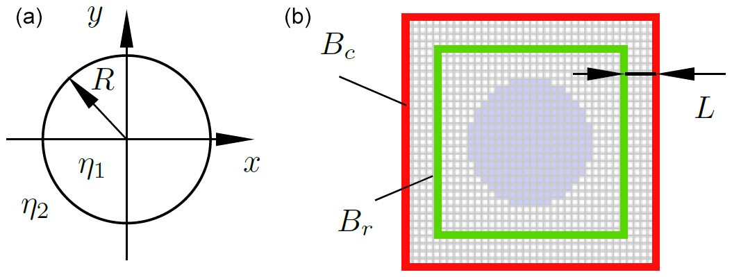
Figure 4(a) Model of a longitudinally infinite and transversely open artificial optical waveguide with η1, η2 being different indices of refraction and R being the radius of the cylindrical waveguide. (b) Two-dimensional rectangular mesh with the reference surface Br and computational domain boundary Bc. Parameters are as follows: Δx=0.4 mm, frequency = 16 GHz, radius R=6.5 mm, L=4 mm, η1=2, η2=1.5.
In order to integrate KIR into the framework of FIT multiple steps are necessary. First, the boundary field values of the computational domain must be replaced by the integral (Eq. 3) along the cell edges. After evaluating the integral, the relationship for a boundary field cell ![]() at the boundary point r is obtained:
at the boundary point r is obtained:
with c0…U being the KI weights and ![]() 0…U,q being the field values at the reference boundary.
0…U,q being the field values at the reference boundary.
In the next step, Eq. (8) will be rearranged so that the values of individual reference sources ![]() i,q can be expressed as a function of the boundary value
i,q can be expressed as a function of the boundary value ![]() x,r and other reference sources.
x,r and other reference sources.
Each row and column of the A matrix from Eq. (7) that corresponds to a specific reference source ![]() i,q must be altered according to Eq. (9), thus a separate matrix AKIR is built up, which consists of the KIR components. This matrix is not sparse, non symmetric, complex-valued and has the same dimensions as the two-dimensional FIT system matrix A from Eq. (7). The structure of the FIT and KIR matrix are shown in Fig. 5.
i,q must be altered according to Eq. (9), thus a separate matrix AKIR is built up, which consists of the KIR components. This matrix is not sparse, non symmetric, complex-valued and has the same dimensions as the two-dimensional FIT system matrix A from Eq. (7). The structure of the FIT and KIR matrix are shown in Fig. 5.
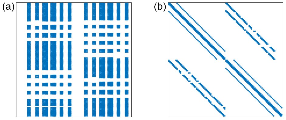
Figure 5(a) Structure of the KIR matrix AKIR. (b) Matrix structure of the two-dimensional FIT eigenvalue problem (Eq. 7).
After AKIR has been set up, it can be integrated into the eigenvalue problem. For this, the AKIR matrix has to be added to the system matrix A:
with AK being the new system matrix of the nonlinear eigenvalue problem.
In order to evaluate the numerical errors of KIR, a representative computational example will be described in this section. In the following examinations, a transversely open cylindrical optical waveguide according to Fig. 4 will be considered. The presented waveguide supports 4 propagating modes which can be calculated analytically (Yeh and Shimabukuro, 2008). Using FIT with KIR, the numerically obtained eigenvalue solution for the monopole TE mode is compared with the analytical solution. This specific monopole mode is chosen, since the azimuthal angle of its field distribution in the transverse plane doesn't change, hence the comparison between the analytical and numerical solutions become easier. The analytical solution of the chosen mode's propagation constant is given by m−1. In order to quantify the field error, the following L2 norm is used:
with , ![]() ,
, ![]() being the analytical and numerical solution, respectively, A being the computational area inside Br and ai being the area of individual cells i. In this particular case of the equidistant mesh in both coordinate directions all ai areas in the computational domain are equal.
being the analytical and numerical solution, respectively, A being the computational area inside Br and ai being the area of individual cells i. In this particular case of the equidistant mesh in both coordinate directions all ai areas in the computational domain are equal.
The boundary formulation presented here has two parameters that can be used to adjust the accuracy and computation cost of the calculation. Both parameters will be introduced in the following subsections. Additionally, a particular KIR for spatially symmetrical structures is discussed.
5.1 Solution of the nonlinear eigenvalue problem
The solution of linearized subsystems of the nonlinear eigenvalue problem can be obtained using a fixed point iteration (FPI), which is used here to calculate individual eigenvalue pairs. The first eigenvalue in Eq. (3) is estimated by the averaged within the iterative solution process, which leads to a sequence of linear eigenvalue problems. Knowing the material properties of the computational domain, known limits for the smallest and highest propagation constants can be specified as
where εi and μi are the relative permittivity and permeability of an individual cell, respectively. Considering a real-valued parameter,
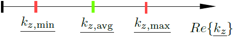
is set to the mean value between and in the initial iteration of the FPI. On the subsequent iterations, is set to one of the obtained solutions. The amount of required iterations depends on the required relative accuracy between individual iterations.
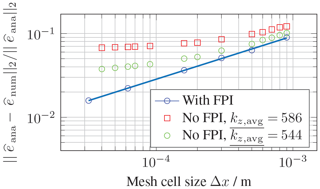
The numerical errors of the eigenvector depend on the difference . The convergence of the FIT model with KIR is shown in Fig. 6, with the L2 error on the ordinate and the mesh cell size on the abscissa. Calculations with FIT result in a convergence order between 1 and 2 if the error is calculated using field integrals. If instead one uses field strength in order to calculate the error, a convergence order between 0.5 and 1 is obtained. In the numerical example specified in Fig. 4 a cylindrical figure is being discretized by a quadratic mesh. Additionally electric field strength is being used to calculate the error. These two reasons lead to the convergence order of 0.51, shown in Fig. 6. Two additional calculations were performed at different fixed and one was conducted using the FPI. In this particular example it is evident, that (i) the error stagnates if no FPI is used and (ii) the error offset is decreasing when is getting closer to the analytical value.
5.2 Distance to the boundary
One of the important parameters is defined as the distance L between the reference contour Br and the boundary Bc as specified in Fig. 4. Changing this value affects the ratio between Rmin, Rmax, which are the closest and furthest distances between the evaluated field on Bc and the reference elements on Bs.
As shown in Fig. 7, the evaluated numerical error increases in two cases: (i) if the distance to the boundary becomes too small, thus the evaluated Green's function gets closer to the singularity and (ii) if the ratio Rmin∕Rmax increases. The choice of an optimal value for L depends on the application.
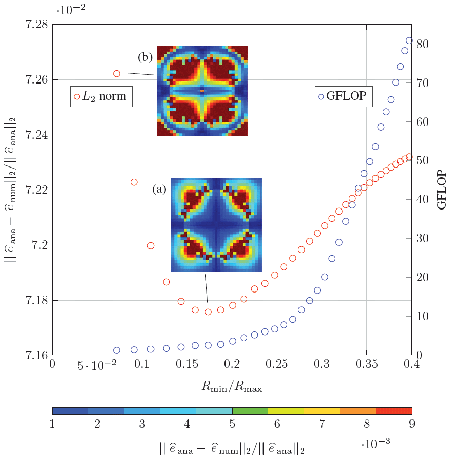
Figure 7Numerical error over the increasing ratio Rmin∕Rmax for the computational example shown in Fig. 4. The distribution of the L2-Error is shown for two calculations in (a) and (b).
Apart from the numerical error, the distance parameter also affects the computational cost. In Fig. 7 the determined amount of floating point operations (FLOP) dependent on the ratio Rmin∕Rmax is shown. Although the adjustment of the distance parameter has a relatively low influence on the overall error, the distribution of the corresponding L2 error shows significant differences.
5.3 KIR for symmetrical structures
Symmetrical waveguides may support modes with a symmetric field distribution with regard to one of the axes of the chosen coordinates. In that case, a dedicated boundary condition can be imposed for the numerical simulation. This reduces the size of the computational domain in the given two-dimensional case by a factor of two of even four depending on the amount of symmetry planes. In case of the example given in Fig. 8 the computational domain can be divided in two parts and only one of those must be taken into account for the calculation. For the selected domain, a dedicated boundary condition must be specified on the dashed symmetry line.
The proposed boundary condition KIR can naturally be used in combination with symmetry-enforcing boundary conditions. However, some implementation details must be particularly considered. Since in case of Fig. 8 one half of the reference sources on Br is missing, these values must be considered using the a priori knowledge of the symmetry. A simplified example in Fig. 9 is used to explain the application of the method. Without the symmetry boundary, for example the value of eA is calculated using:
with rn as the distance between the edge n and the edge A and f(rn) as the function calculating the weights of the Kirchhoff-Integral. Field values e7–e12 can be calculated using the knowledge of the values e1–e6 and the waveguide symmetry.
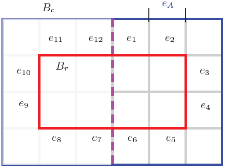
Figure 9Schematic of a model with a possible symmetry plane and its implication on the field evaluation formulation.
Using a symmetry boundary condition leads to a reduction of the system matrix by the factor of two.
5.4 Reduction of reference sources
The evaluation of the Kirchhoff Integral requires the integration over a closed surface. If the reference point is close to the respective surface, only a small fraction of the entire surface may contribute to the value on account of the weighting with the Green's functions kernel. If this situation holds, considering a fraction of the entire surface is sufficient to obtain an adequate solution.
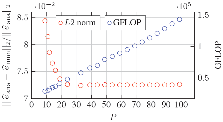
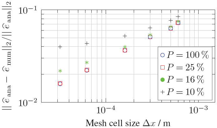
Another KIR parameter, further referred to as parameter P defines the amount of reference sources in percentage used for evaluating an individual field value. On the one hand, the overall computational cost decreases with the number of reference sources. On the other hand, lower values of P leads to a higher numerical error (see Fig. 10). Similar investigations in form of a convergence study also shows the dependency on the fraction of the considered reference sources as can be seen in Fig. 11. For this particular example it is recognizable, that considered reference sources between 25 % and 100 % show a similar convergence behavior. The intentionally introduced reduction of reference sources leads to a smaller amount of DoF in the system matrix specified in Eq. (7), which in turn decreases the overall computational cost as expected.
The presented KIR boundary representation contains three types of approximations that will be addressed in this sections:
-
numerical derivative of the electric field strength;
-
numerical integration of the electric field strength;
-
numerical integration of the Green's function.
6.1 Numerical derivative of the electric field strength
The evaluation of the Kirchhoff Integral (Eq. 3) requires the calculation of a derivative of the electric field strength. In order to evaluate this quantity numerically within the framework of FIT, a central differential quotient is used:
The order of this approximation is 𝒪(Δx2), which is the same for FIT in the used formulation with field integrals as eigenvector components. Since this approximation depends on the mesh size, it is not possible to analyze its sole influence on the overall convergence rate independently because changing the mesh size will also affect the approximations of FIT.
6.2 Numerical integration of the electric field strength
The Kirchhoff Integral (Eq. 3) allows the evaluation of the electric field strength at any position in a given region. However, for the used FIT formulation, integrals of electric fields are required, as described in Sect. 3.2. Thus, a numerical integration of the result is needed, which is simply achieved by the midpoint rule:
The approximation error here is also 𝒪(Δx2), which is again the same for FIT in the used formulation with field integrals as eigenvector components. Just like the approximation of the derivative, here it is also not possible to analyze the sole influence of this error on the overall convergence rate.
6.3 Numerical integration of the Green's function
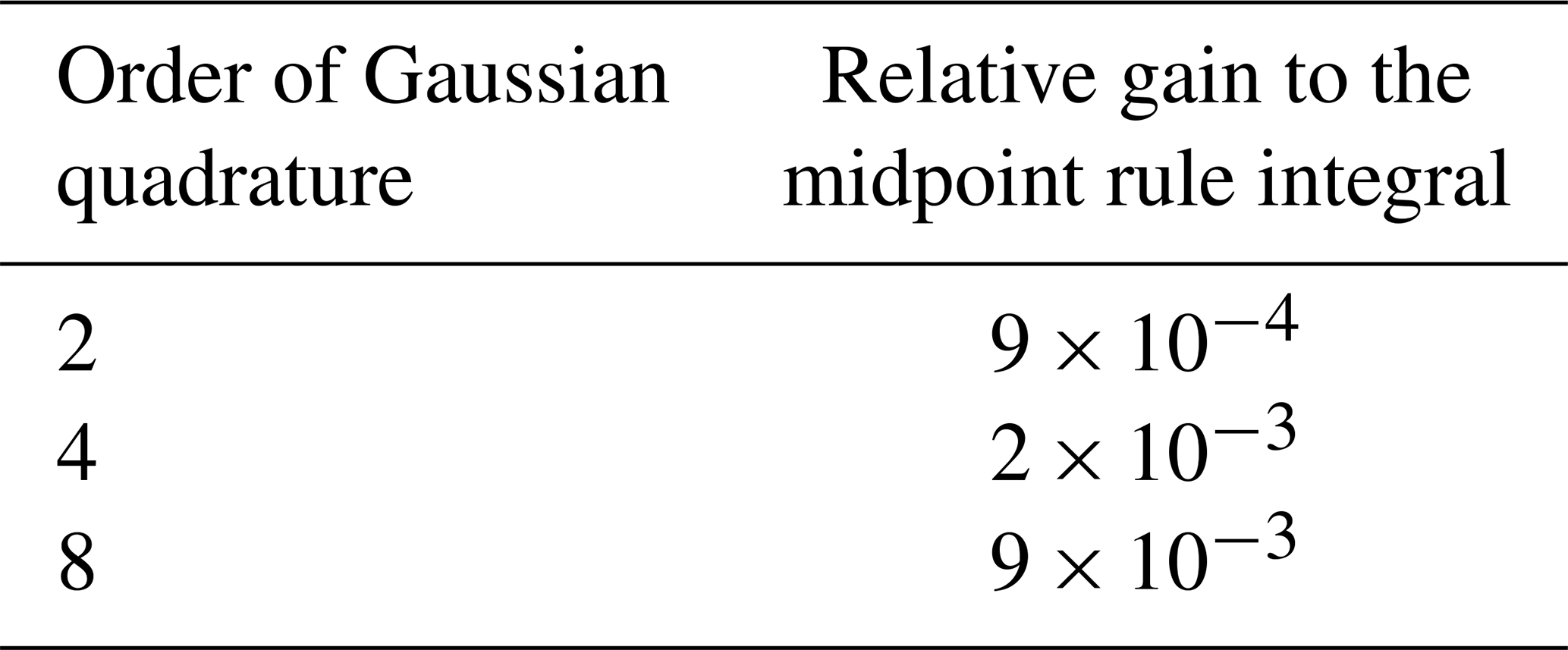
In the one-dimensional Kirchhoff Integral (Eq. 3) both, the electric field strength and the Green's function are integrated over a contour C. The integration over an individual cell edge with an assumed constant field quantity allows to pull out the electric field from the actual integral. Hence, the remaining Green's function and its derivative can be integrated separately. For example by using the Gaussian quadrature (Stoer, 2005). The error for a Gaussian quadrature of the order 2n+2 is defined as
with
and
This approximation can be evaluated independent of the mesh cell size. Using the example described in Sect. 4, the L2 error was calculated with Gaussian quadrature orders n=2, 4, 8. In Table 1, selected results are displayed as a relative difference to the midpoint rule integral. The accuracy gain between the midpoint rule and higher order Gaussian quadrature is relatively low, as this example shows.
Table 1L2 error for different orders of Gaussian quadrature for the numerical integration of the Green's function. The relative gain is defined as , with fg and fm being the solution using Gaussian quadrature and midpoint rule respectively.
In this section, the presented KIR boundary is compared with closed and absorbing boundaries PEC, PMC and PML. All required algorithms were implemented within the framework of FIT in a custom MATLAB® code. The PML was realized as a uniaxial PML (UPML) as described in Tischler (2004). In order to compare different boundary conditions with each other, three different computational examples are examined.
First, the numerical solution and its error is obtained using KIR. Next, the distance to the boundary is varied such that the same eigenvector accuracy, defined by the L2 norm (Eq. 10) is obtained for PEC, PMC and PML termination. Compared quantities are given by the distance between both boundaries, the amount of degrees of freedom (DoF), the amount of FLOP, the amount of nonzero elements (NZE) in the eigenvalue matrix and the amount of mesh cells.
7.1 Transmission line
A transversely open double cylindrical wire transmission line as show in Fig. is used as the first application. For this configuration an analytical solution for the TEM mode with exists and is used as a reference solution. In Table 2 the simulation results obtained are summarized and it is apparent that the KIR boundary uses less DoF and less cells then the other examined types of boundaries. For this calculation with KIR only one FPI step was needed, since the only existing propagation mode in this example is know in advance. The solution obtained with PEC shows a higher distance between boundaries Br and Bc than in the case with PMC. This is due to the fact, that the PEC boundary introduces an additional conductor, which distorts the physical model.
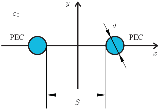
Figure 12Layout of an open two-wire transmission line. Parameters are as follows: mesh cell size Δx=0.3 mm, frequency = 16 GHz, diameter d=3 mm, distance S=12 mm.
Table 2Comparison between different boundary conditions used to terminate the transmission line model from Fig. as a computational example. This shows that the computational effort needed for the simulation is lower for the calculation performed using KIR.
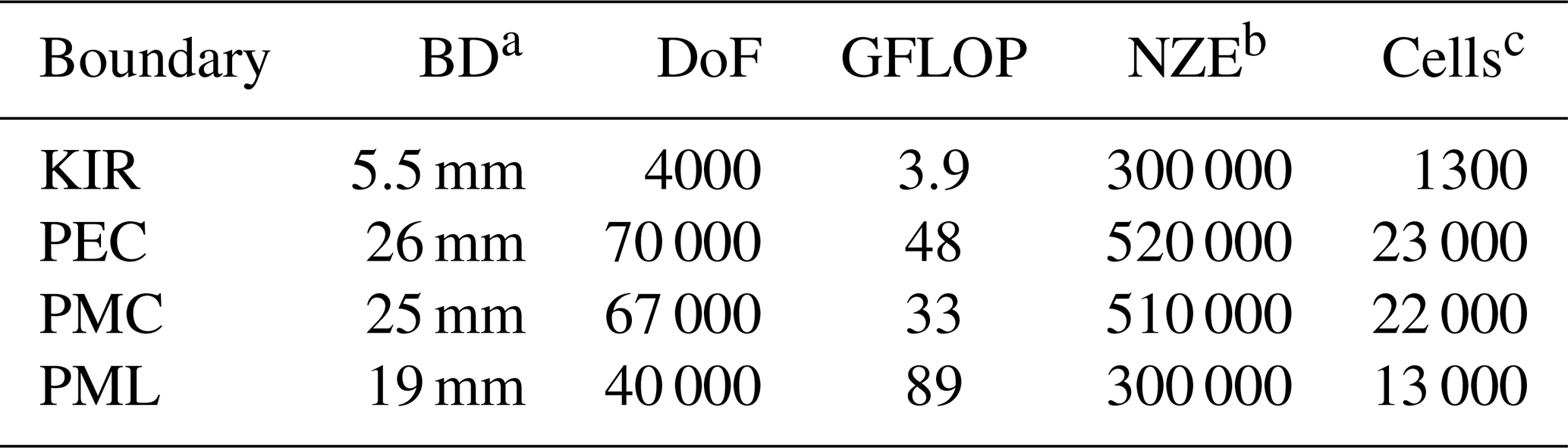
a Distance between boundaries Br and Bc. b Number of Non-Zero-Elements. c Amount of cells.
7.2 Optical waveguide
An uncoated optical waveguide as shown in in Fig. 4 is considered in the second application example. The model itself is described in Sect. 4.
Results for the comparison between different boundary conditions with the KIR boundary is shown in the Table 3. For this calculation with KIR two FPI steps were needed. Two iterations were needed to reach the solution with KIR. Although the amount of FLOP for calculations with PEC and KIR boundaries are equal, the amount of DoF differs by the factor of 2.5. What is more important is the fact, that the obtained solution spectrum with the PEC boundary is polluted with modes that do not correspond to the initial physical model.
Table 3Comparison between different boundary conditions used to terminate the optical waveguide from Fig. 4 as a computational example. This shows that the computational effort needed for the simulation is lower for the calculation performed using KIR.
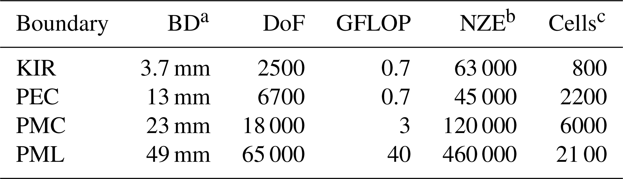
a Distance between boundaries Br and Bc. b Number of Non-Zero-Elements. c Amount of cells.
7.3 Microstrip line
A microstrip line, displayed in Fig. 13 is used as a representative example. Since no analytical solution for this problem can be found, a numerical reference solution was calculated using the commercial CEM Software CST MICROWAVE STUDIO®. For the comparison the quasi TEM mode is chosen here.
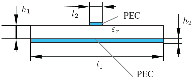
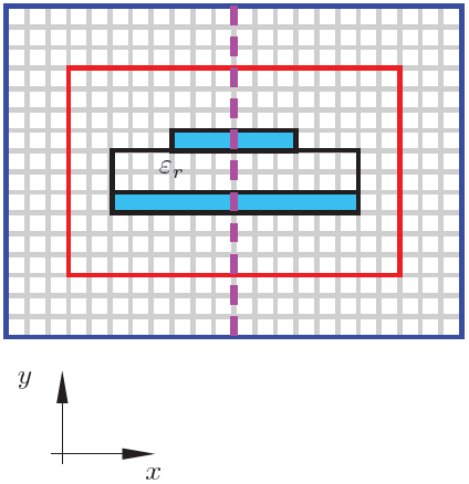
Figure 13Microstrip line with a dielectric substrate and PEC elements. Following parameters for this model are used: h1=0.12 mm, h2=0.012 mm, l1=1.2 mm, l2=0.12 mm, εr=4, mesh width Δx=0.012 mm, frequency = 16 GHz.
In Table 4 the compiled results show that the model with the KIR boundary requires less DoF and less mesh cells than the other models calculated using classical boundaries on the microstrip line described above. For this calculation with KIR one FPI step was needed. The solution obtained with the PMC model shows computational costs in the same order of magnitude as the one, calculated using KIR. Nevertheless, with the remaining boundaries the eigenvalue spectrum contains modes that do not exist in the transversely open waveguide (e.g. complex modes).
Table 4Comparison between different boundary conditions used to terminate the microstrip line from Fig. 13 as a computational example. This shows that the computational effort needed for the simulation is lower for the calculation performed using KIR.
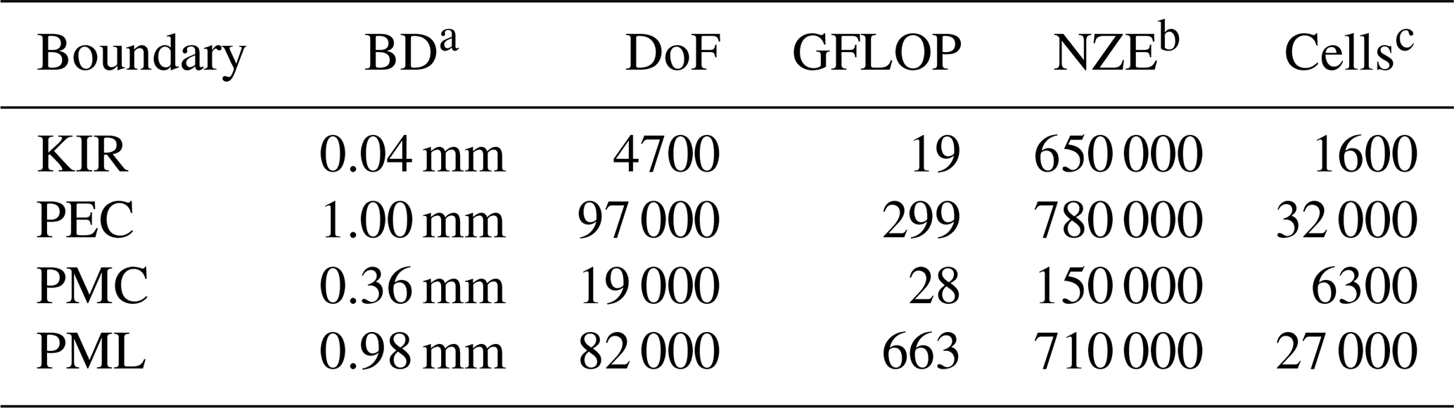
a Distance between boundaries Br and Bc. b Number of Non-Zero-Elements. c Amount of cells.
An alternative boundary condition KIR for transversally open waveguides was defined and successfully implemented within the framework of FIT. Various parameters and approximations of KIR were introduced and discussed. Finally, a comparison between conventional boundary conditions and KIR was performed. In contrast to classical boundary conditions, KIR representation results in a better approximation of the physical problem. This significantly lowers the computation time.
All the calculations performed for this paper (besides the one calculated using CST MICROWAVE STUDIO) were calculated using a custom MATLAB code. Neither the CST code nor the MATLAB code are publicly available. Also the underlying data is not publicly available – only the research data displayed in this paper.
The supplement related to this article is available online at: https://doi.org/10.5194/ars-18-7-2020-supplement.
MP has conceived, designed and performed the analysis, collected the data and written the paper. WA has assisted in the analysis and the finalization of the paper. TW has assisted in the analysis and the finalization of the paper.
The authors declare that they have no conflict of interest.
This article is part of the special issue “Kleinheubacher Berichte 2019”. It is a result of the Kleinheubacher Berichte 2019, Miltenberg, Germany, 23–25 September 2019.
This paper was edited by Thomas Eibert and reviewed by two anonymous referees.
Bandlow, B., Sievers, D., and Schuhmann, R.: An Improved Jacobi-Davidson Method for the Computation of Selected Eigenmodes in Waveguide Cross Sections, IEEE T. Magnet., 46, 3461–3464, https://doi.org/10.1109/TMAG.2010.2046315, 2010. a
Bérenger, J. P.: A perfectly matched layer for the absorption of electromagnetic waves, J. Comput. Phys., 114, 185–200, 1994. a
Clarricoats, P. J. B. and Slinn, K. R.: Complex modes of propagation in dielectric-loaded circular waveguide, Electron. Lett., 1, 145–146, https://doi.org/10.1049/el:19650137, 1965. a
Jabłoński, T. F.: Complex modes in open lossless dielectric waveguides, J. Opt. Soc. Am. A, 11, 1272–1282, 1994. a
Jackson, J. D.: Classical Electrodynamics, 3rd Edn., Wiley, 1998. a, b, c, d
Johnson, S. G.: Notes on Perfectly Matched Layers (PMLs), in: Lecture notes, Massachusetts Institute of Technology, Massachusetts, March 2010. a
Monsoriu, J. A., Coves, A., Gimeno, B., Andres, M. V., and Silvestre, E.: A robust and efficient method for obtaining the complex modes in inhomogeneously filled waveguides, Microw. Opt. Technol. Lett., 37, 218–222, https://doi.org/10.1002/mop.10875, 2003. a
Roden, J. A. and Gedney, S. D.: Convolution PML (CPML): An efficient FDTD implementation of the CFS–PML for arbitrary media, Microw. Opt. Technol. Lett., 27, 334–339, https://doi.org/10.1002/1098-2760(20001205)27:5<334::AID-MOP14>3.0.CO;2-A, 2000. a
Rogier, H. and De Zutter, D.: Berenger and leaky modes in microstrip substrates terminated by a perfectly matched layer, IEEE T. Microw. Theory Tech., 49, 712–715, https://doi.org/10.1109/22.915446, 2001. a
Schmitt, D.: Zur numerischen Berechnung von Resonatoren und Wellenleitern, Diss., Technische Universität Darmstadt, Darmstadt, July 1994. a
Stoer, J.: Numerische Mathematik 1, Springer, 2005. a
Strube J. and Arndt, F.: Rigorous Hybrid-Mode Analysis of the Transition from Rectangular Waveguide to Shielded Dielectric Image Guide, IEEE T. Microw. Theory Tech., 33, 391–401, https://doi.org/10.1109/TMTT.1985.1133010, 1985. a
Talukder, P. K.: Finite-Difference-Frequency-Domain Simulation of Electrically Large Microwave Structures using PML and Internal Ports, Diss., Technische Universität Berlin, Berlin, January 2009. a
Tischler, T.: Die Perfectly-Matched-Layer-Randbedingung in der Finite-Differenzen-Methode im Frequenzbereich: Implementierung und Einsatzbereiche, Diss., Technische Universität Berlin, Berlin, December 2004. a
Weiland, T.: A Discretisation Method for the Solution of Maxwells Equations for six-Component Fields, Electron. Commun., 31, 116–120, 1977. a, b
Weiland, T.: Electromagnetic simulators – status and future directions, IET Sci. Meas. Technol., 11, 681–686, 2017. a
Yeh, C. and Shimabukuro, F.: The Essence of Dielectric Waveguides, Springer Science + Business Media, LLC, 137–145, 2008. a
Symbols consisting of letters and bows might not be displayed correctly in this version of the published article.
- Abstract
- Introduction
- Conventional solutions
- Enhanced solution approach
- Computational examples
- Investigation of KIR properties
- Sources of KIR approximations
- Applications of KIR
- Conclusions
- Data availability
- Author contributions
- Competing interests
- Special issue statement
- Review statement
- References
- Supplement