Reconstruction of signal phases for signals closer than the DFT frequency resolution

Radar signal processing is a promising tool for vital sign monitoring. For contactless observation of breathing and heart rate a precise measurement of the distance between radar antenna and the patient's skin is required. This results in the need to detect small movements in the range of 0.5 mm and below. Such small changes in distance are hard to be measured with a limited radar bandwidth when relying on the frequency based range detection alone. In order to enhance the relative distance resolution a precise measurement of the observed signal's phase is required. Due to radar reflections from surfaces in close proximity to the main area of interest the desired signal of the radar reflection can get superposed. For superposing signals with little separation in frequency domain the main lobes of their discrete Fourier transform (DFT) merge into a single lobe, so that their peaks cannot be differentiated. This paper evaluates a method for reconstructing the phase and amplitude of such superimposed signals.

1 Introduction

Radar appliances are a promising platform for contactless vital sign monitoring. Due to regulations the usable bandwidth and hence the distance resolution is limited. With signal analysis based on the Fourier transform this results in limitations of the maximum achievable frequency and distance resolution. Algorithms like estimation of signal parameters via rotational invariance techniques (ESPRIT) or MUltiple SIgnal Classification (MUSIC) allow detection of signal frequencies with much closer limits. They provide frequency estimates or a pseudospectrum, that can be used for peak detection. While those methods provide good signal separation in frequency domain, they do not provide values for signal phase or amplitude. Figure 1 shows the observation of a pair of oscillations, that have similar frequencies.

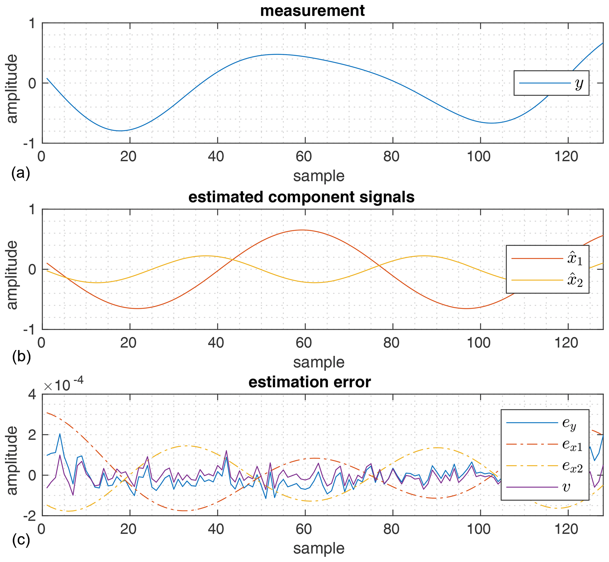
Figure 1 Superposition of signals with similar signal frequencies and their reconstruction in time domain: (a) shows the signal measurement y is shown. Based on this measurement the component signals ${\widehat{x}}_{\mathrm{1}}$ and ${\widehat{x}}_{\mathrm{2}}$ shown in (b) are estimated. With this the measurement error $e_y=y\mathrm{-}{\widehat{x}}_{\mathrm{1}}\mathrm{-}{\widehat{x}}_{\mathrm{2}}$ is determined in (c). The actual signal noise v, that was used for generating the measurement y, is also shown for comparison.

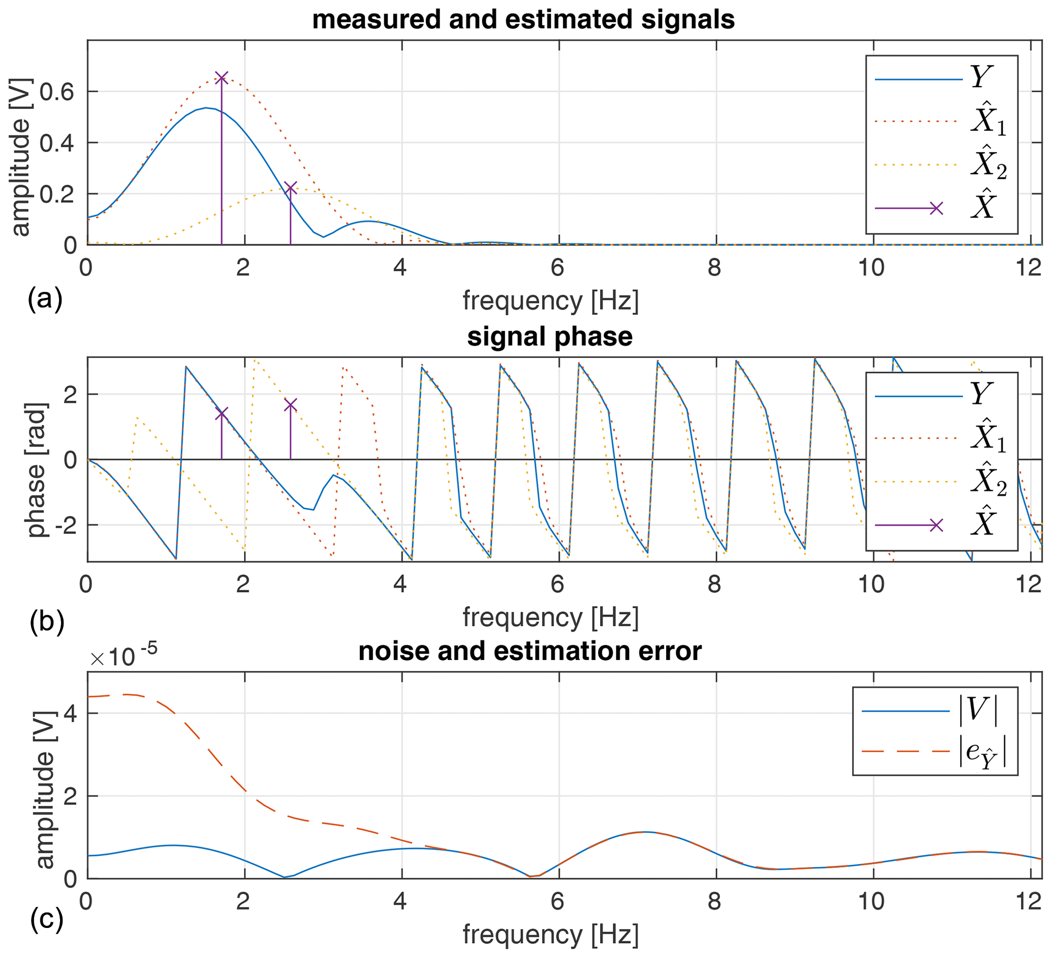
Figure 2 Superposition of two signals x₁ and x₂, that are similar in frequency: (a) shows the power spectral density (PSD) of the measured signal Y and the signal signal noise V. The dotted lines show the PSD in (a) and phase of the matching estimated signals ${\widehat{X}}_{\mathrm{1}}$ and ${\widehat{X}}_{\mathrm{2}}$ in (b). The crosses $\widehat{X}$ show amplitude and phase estimates based on the frequency values delivered by an ESPRIT total least squares algorithm. The dashed line in (c) shows the residual error e_y, when the signal estimates ${\widehat{X}}_{\mathrm{1}}$ and ${\widehat{X}}_{\mathrm{2}}$ are subtracted from the observed signal.

The corresponding power spectral densities (PSD) displayed in Fig. 2 make the difficulty in determining the correct signal frequencies obvious.

Section 2 presents a way to retrieve the signals' amplitude and phase based on a harmonic signal model, assuming the signals' frequencies can be estimated. The presented method is evaluated in Sect. 3 before a conclusion is discussed in Sect. 4.

2 Signal parameter estimation

For a successful phase and amplitude reconstruction an accurate signal model is required. Using a matrix representation of superimposed harmonic signals as described in Sect. 2.1 forms the basis for frequency, phase and amplitude estimation. For the analysis presented in this paper the signal frequencies are determined using estimation of signal parameters via rotational invariance techniques (ESPRIT). However any algorithm could be used, that allows a reasonably precise estimation of signal frequencies. Therefore only the general principle of ESPRIT is described in Sect. 2.2. The phase and amplitude estimation is done using the method described in Sect. 2.3.

2.1 Harmonic signal model

A sampled harmonic oscillation x_p is completely described by its amplitude a_p, frequency f_p and its initial phase value Φ_p as a function of time t:

$$\begin{array}{}\text{(1)}& x_p\left(t\right)=a_p\cos \left(\mathrm{2}\mathit{\pi }{f}_p\cdot t+{\mathrm{\Phi }}_p\right)\end{array}$$

In discrete signal processing any signal is sampled using a finite sampling frequency $F_{\mathrm{s}}=\frac{\mathrm{1}}{T}$. It can be described in multiple equivalent equations:

$$\begin{array}{ll}\text{(2)}& {\displaystyle }{x}_p\left(n\right)& {\displaystyle }={\displaystyle \frac{\mathrm{1}}{\mathrm{2}}}\left[{\underset{\mathrm{¯}}{x}}_p+{\underset{\mathrm{¯}}{x}}_p^{*}\right]\text{(3)}& {\displaystyle }& {\displaystyle }={\displaystyle \frac{\mathrm{1}}{\mathrm{2}}}\left[a_p{e}^{j\mathrm{2}\mathit{\pi }{f}_p\cdot T\cdot n+{\mathrm{\Phi }}_p}+a_p{e}^{-j\mathrm{2}\mathit{\pi }{f}_p\cdot T\cdot n-{\mathrm{\Phi }}_p}\right]\text{(4)}& {\displaystyle }& {\displaystyle }=a_p\cos \left(\mathrm{2}\mathit{\pi }{f}_p\cdot T\cdot n+{\mathrm{\Phi }}_p\right)\text{(5)}& {\displaystyle }& {\displaystyle }=a_p[\cos \left(\mathrm{2}\mathit{\pi }{f}_{p}Tn\right)\cos \left({\mathrm{\Phi }}_p\right){\displaystyle }& {\displaystyle }-\sin \left(\mathrm{2}\mathit{\pi }{f}_{p}Tn\right)\sin \left({\mathrm{\Phi }}_p\right)]\end{array}$$

The superposition of P complex signals ${\underset{\mathrm{¯}}{x}}_p\left(n\right)$

$$\begin{array}{}\text{(6)}& \underset{\mathrm{¯}}{x}\left(n\right)=\stackrel{P}{\sum _{p=\mathrm{1}}}{\underset{\mathrm{¯}}{x}}_p\left(n\right)\end{array}$$

can be described as follows:

$$\begin{array}{}\text{(7)}& {\displaystyle }{\underset{\mathrm{¯}}{a}}_p=a_p\cdot e^{j{\mathrm{\Phi }}_p}\text{(8)}& {\displaystyle }{\underset{\mathrm{¯}}{b}}_p\left(n\right)=e^{j\mathrm{2}\mathit{\pi }{f}_p\cdot T\cdot n}\text{(9)}& {\displaystyle }\Rightarrow \underset{\mathrm{¯}}{x}\left(n\right)=\stackrel{P}{\sum _{p=\mathrm{1}}}{\underset{\mathrm{¯}}{a}}_p\cdot {\underset{\mathrm{¯}}{b}}_p\left(n\right)\end{array}$$

For real valued signals this expression expands to:

$$\begin{array}{ll}\text{(10)}& {\displaystyle }x\left(n\right)=& {\displaystyle }\stackrel{P}{\sum _{p=\mathrm{1}}}{\displaystyle \frac{\mathrm{1}}{\mathrm{2}}}\left[{\underset{\mathrm{¯}}{a}}_p\cdot {\underset{\mathrm{¯}}{b}}_p\left(n\right)+{\underset{\mathrm{¯}}{a}}_p^{*}\cdot {\underset{\mathrm{¯}}{b}}_p^{*}\left(n\right)\right]\text{(11)}& {\displaystyle }=& {\displaystyle }\stackrel{P}{\sum _{p=\mathrm{1}}}{a}_p[\cos \left({\mathrm{\Phi }}_p\right)\cdot \cos \left(\mathrm{2}\mathit{\pi }{f}_{p}Tn\right){\displaystyle }& {\displaystyle }-\sin \left({\mathrm{\Phi }}_p\right)\cdot \sin \left(\mathrm{2}\mathit{\pi }{f}_{p}Tn\right)]\end{array}$$

2.2 Frequency estimation

For the analysis in this paper frequency estimation is done using ESPRIT. Since the method of frequency estimation is exchangeable and not the main scope of this paper, only a rough outline of the ESPRIT algorithm is given in this section (Roy and Kailath, 1989; Ingle et al., 2005).

Based on the harmonic signal model the signal vectors ${\underset{\mathrm{¯}}{\mathit{x}}}_p$ can be defined

$$\begin{array}{}\text{(12)}& {\underset{\mathrm{¯}}{\mathit{x}}}_p={\left[\begin{array}{cccc}{\underset{\mathrm{¯}}{x}}_p\left(\mathrm{0}\right)& {\underset{\mathrm{¯}}{x}}_p\left(\mathrm{1}\right)& \mathrm{\dots }& {\underset{\mathrm{¯}}{x}}_p(N-\mathrm{1})\end{array}\right]}^{\mathrm{T}}\end{array}$$

such that a composite signal matrix $\underset{\mathrm{¯}}{X}$ can be formed:

$$\begin{array}{}\text{(13)}& \underset{\mathrm{¯}}{\mathbf{X}}=\left[\begin{array}{cccc}{\underset{\mathrm{¯}}{\mathit{x}}}_{\mathrm{1}}& {\underset{\mathrm{¯}}{\mathit{x}}}_{\mathrm{2}}& \mathrm{\dots }& {\underset{\mathrm{¯}}{\mathit{x}}}_P\end{array}\right]\end{array}$$

By splitting the signal matrix $\underset{\mathrm{¯}}{X}$ into submatrices

$$\begin{array}{}\text{(14)}& {\displaystyle }{\underset{\mathrm{¯}}{\mathbf{X}}}_{\mathrm{1}}=& {\displaystyle }\left[\begin{array}{cc}{\mathbf{I}}_{N-\mathrm{1}}& \mathbf{0}\end{array}\right]\underset{\mathrm{¯}}{\mathbf{X}}\text{(15)}& {\displaystyle }=& {\displaystyle }\left[\begin{array}{cccc}{\underset{\mathrm{¯}}{x}}_{\mathrm{1}}\left(\mathrm{0}\right)& {\underset{\mathrm{¯}}{x}}_{\mathrm{2}}\left(\mathrm{0}\right)& \mathrm{\dots }& {\underset{\mathrm{¯}}{x}}_p\left(\mathrm{0}\right)\\ {\underset{\mathrm{¯}}{x}}_{\mathrm{1}}\left(\mathrm{1}\right)& {\underset{\mathrm{¯}}{x}}_{\mathrm{2}}\left(\mathrm{1}\right)& \mathrm{\dots }& {\underset{\mathrm{¯}}{x}}_p\left(\mathrm{1}\right)\\ \mathrm{⋮}& \mathrm{⋮}& \mathrm{\ddots }& \mathrm{⋮}\\ {\underset{\mathrm{¯}}{x}}_{\mathrm{1}}(N-\mathrm{2})& {\underset{\mathrm{¯}}{x}}_{\mathrm{2}}(N-\mathrm{2})& \mathrm{\dots }& {\underset{\mathrm{¯}}{x}}_p(N-\mathrm{2})\end{array}\right]\end{array}$$

and

$$\begin{array}{}\text{(16)}& {\displaystyle }{\underset{\mathrm{¯}}{\mathbf{X}}}_{\mathrm{2}}=& {\displaystyle }\left[\begin{array}{cc}\mathbf{0}& {\mathbf{I}}_{N-\mathrm{1}}\end{array}\right]\mathbf{X}\text{(17)}& {\displaystyle }=& {\displaystyle }\left[\begin{array}{cccc}{\underset{\mathrm{¯}}{x}}_{\mathrm{1}}\left(\mathrm{1}\right)& {\underset{\mathrm{¯}}{x}}_{\mathrm{2}}\left(\mathrm{1}\right)& \mathrm{\dots }& {\underset{\mathrm{¯}}{x}}_p\left(\mathrm{1}\right)\\ {\underset{\mathrm{¯}}{x}}_{\mathrm{1}}\left(\mathrm{2}\right)& {\underset{\mathrm{¯}}{x}}_{\mathrm{2}}\left(\mathrm{2}\right)& \mathrm{\dots }& {\underset{\mathrm{¯}}{x}}_p\left(\mathrm{2}\right)\\ \mathrm{⋮}& \mathrm{⋮}& \mathrm{\ddots }& \mathrm{⋮}\\ {\underset{\mathrm{¯}}{x}}_{\mathrm{1}}(N-\mathrm{1})& {\underset{\mathrm{¯}}{x}}_{\mathrm{2}}(N-\mathrm{1})& \mathrm{\dots }& {\underset{\mathrm{¯}}{x}}_p(N-\mathrm{1})\end{array}\right]\end{array}$$

the signal frequencies f_p are embedded into the diagonal matrix Φ

$$\begin{array}{}\text{(18)}& \mathbf{\Phi }=\mathrm{diag}\left[\begin{array}{cccc}{e}^{j\mathrm{2}\mathit{\pi }{f}_{\mathrm{1}}T}& e^{j\mathrm{2}\mathit{\pi }{f}_{\mathrm{2}}T}& \mathrm{\dots }& e^{j\mathrm{2}\mathit{\pi }{f}_{P}T}\end{array}\right]\end{array}$$

, that relates both signal matrices ${\underset{\mathrm{¯}}{\mathbf{X}}}_{\mathrm{1}}$ and${\underset{\mathrm{¯}}{\mathbf{X}}}_{\mathrm{2}}$:

$$\begin{array}{}\text{(19)}& {\underset{\mathrm{¯}}{\mathbf{X}}}_{\mathrm{2}}={\underset{\mathrm{¯}}{\mathbf{X}}}_{\mathrm{1}}\mathbf{\Phi }\end{array}$$

Because the actual signals ${\underset{\mathrm{¯}}{x}}_p$ and the corresponding signal matrix $\underset{\mathrm{¯}}{\mathbf{X}}$ are unknown in real applications, for the ESPRIT algorithm a measured signal vector $\mathit{y}=\left[\begin{array}{cccc}y\left(\mathrm{0}\right)& y\left(\mathrm{1}\right)& \mathrm{\dots }& y(N-\mathrm{1})\end{array}\right]$ is rearranged to generate a data matrix

$$\begin{array}{}\text{(20)}& \mathbf{Y}=\left[\begin{array}{cccc}y\left(\mathrm{0}\right)& y\left(\mathrm{1}\right)& \mathrm{\dots }& y(M-\mathrm{1})\\ y\left(\mathrm{1}\right)& y\left(\mathrm{2}\right)& \mathrm{\dots }& y\left(M\right)\\ \mathrm{⋮}& \mathrm{⋮}& \mathrm{\ddots }& \mathrm{⋮}\\ y(N-M)& y(N-M+\mathrm{1})& \mathrm{\dots }& y(N-\mathrm{1})\end{array}\right]\end{array}$$

. This data matrix is used for singular value decomposition

$$\begin{array}{}\text{(21)}& \mathbf{Y}=\mathbf{L}\mathbf{\Sigma }{\mathbf{U}}^{\mathrm{H}}\end{array}$$

in order to get the signal subspace ${\mathbf{U}}_{\mathrm{s}}^{\mathrm{H}}$ from U^H. The signal subspace U_s itself is split into

$$\begin{array}{}\text{(22)}& {\underset{\mathrm{¯}}{\mathbf{U}}}_{\mathrm{1}}=\left[\begin{array}{cc}{\mathbf{I}}_{P-\mathrm{1}}& \mathbf{0}\end{array}\right]{\mathbf{U}}_{\mathrm{s}}\end{array}$$

and

$$\begin{array}{}\text{(23)}& {\underset{\mathrm{¯}}{\mathbf{U}}}_{\mathrm{2}}=\left[\begin{array}{cc}\mathbf{0}& {\mathbf{I}}_{P-\mathrm{1}}\end{array}\right]{\mathbf{U}}_{\mathrm{s}},\end{array}$$

so that both matrices are related by the rotation matrix Ψ:

$$\begin{array}{}\text{(24)}& {\mathbf{U}}_{\mathrm{2}}={\mathbf{U}}_{\mathrm{1}}\mathbf{\Psi }\end{array}$$

The eigenvalues of Ψ correspond to the values in the diagonal matrix Φ, so that the component signal frequencies f_p can be acquired.

2.3 Phase and amplitude reconstruction

The signal model presented in Sect. 2.1 and a reasonably good estimate of the signal frequencies give the prerequisites for phase and amplitude reconstruction. By writing Eq. (9) as a matrix operation relating the signal vector $\underset{\mathrm{¯}}{\mathit{x}}$

$$\begin{array}{}\text{(25)}& \underset{\mathrm{¯}}{\mathit{x}}={\left[\begin{array}{ccccc}\underset{\mathrm{¯}}{x}\left(\mathrm{0}\right)& \underset{\mathrm{¯}}{x}\left(\mathrm{1}\right)& \mathrm{\dots }& \underset{\mathrm{¯}}{x}(N-\mathrm{2})& \underset{\mathrm{¯}}{x}(N-\mathrm{1})\end{array}\right]}^{\mathrm{T}}\end{array}$$

and complex amplitude vector $\underset{\mathrm{¯}}{\mathit{a}}$

$$\begin{array}{}\text{(26)}& \underset{\mathrm{¯}}{\mathit{a}}={\left[\begin{array}{ccccc}{\underset{\mathrm{¯}}{a}}_{\mathrm{1}}& {\underset{\mathrm{¯}}{a}}_{\mathrm{1}}^{*}& \mathrm{\dots }& {\underset{\mathrm{¯}}{a}}_P& {\underset{\mathrm{¯}}{a}}_P^{*}\end{array}\right]}^{\mathrm{T}}\end{array}$$

a simple matrix operation can be used to describe the sum of an arbitrary number of harmonic oscillations:

$$\begin{array}{}\text{(27)}& \underset{\mathrm{¯}}{\mathit{x}}=\underset{\mathrm{¯}}{\mathbf{B}}\cdot \underset{\mathrm{¯}}{\mathit{a}}\end{array}$$

With the condition of a known sampling time T and known signal frequencies f_p the matrix $\underset{\mathrm{¯}}{\mathbf{B}}$ is defined according to Eq. (8) for an observation window of N samples:

$$\begin{array}{}\text{(28)}& \underset{\mathrm{¯}}{\mathbf{B}}=\left[\begin{array}{cccc}{\underset{\mathrm{¯}}{b}}_{\mathrm{1}}\left(\mathrm{0}\right)& {\underset{\mathrm{¯}}{b}}_{\mathrm{2}}\left(\mathrm{0}\right)& \mathrm{\dots }& {\underset{\mathrm{¯}}{b}}_P\left(\mathrm{0}\right)\\ {\underset{\mathrm{¯}}{b}}_{\mathrm{1}}\left(\mathrm{1}\right)& {\underset{\mathrm{¯}}{b}}_{\mathrm{2}}\left(\mathrm{1}\right)& \mathrm{\dots }& {\underset{\mathrm{¯}}{b}}_P\left(\mathrm{1}\right)\\ \mathrm{⋮}& \mathrm{⋮}& \mathrm{\ddots }& \mathrm{⋮}\\ {\underset{\mathrm{¯}}{b}}_{\mathrm{1}}(N-\mathrm{1})& {\underset{\mathrm{¯}}{b}}_{\mathrm{2}}(N-\mathrm{1})& \mathrm{\dots }& {\underset{\mathrm{¯}}{b}}_P(N-\mathrm{1})\end{array}\right]\end{array}$$

Similarly Eq. (11) can be written as a real valued matrix operation relating the signal vector x and a real valued amplitude vector a:

$$\begin{array}{}\text{(29)}& \mathit{x}=\mathbf{B}\cdot \mathit{a}\end{array}$$

In this case the amplitude vector becomes a composite of the in-phase and the quadrature amplitude values a_p,I and a_p,Q:

$$\begin{array}{}\text{(30)}& \mathit{a}={\left[\begin{array}{ccccc}{a}_{\mathrm{1},\mathrm{I}}& a_{\mathrm{1},\mathrm{Q}}& \mathrm{\dots }& a_{P,\mathrm{I}}& a_{P,\mathrm{Q}}\end{array}\right]}^{\mathrm{T}}\end{array}$$

The real valued matrix B is defined defined as:

$$\begin{array}{}\text{(31)}& \begin{array}{rl}\mathbf{B}=& \left[\begin{array}{ccc}\cos \left(\mathrm{2}\mathit{\pi }{f}_{\mathrm{1}}T\cdot \mathrm{0}\right)& \sin \left(\mathrm{2}\mathit{\pi }{f}_{\mathrm{1}}T\cdot \mathrm{0}\right)& \mathrm{\cdots }\\ \cos \left(\mathrm{2}\mathit{\pi }{f}_{\mathrm{1}}T\cdot \mathrm{1}\right)& \sin \left(\mathrm{2}\mathit{\pi }{f}_{\mathrm{1}}T\cdot \mathrm{1}\right)& \mathrm{\cdots }\\ \mathrm{⋮}& \mathrm{⋮}& \mathrm{\ddots }\\ \cos \left(\mathrm{2}\mathit{\pi }{f}_{\mathrm{1}}T\cdot [N-\mathrm{1}]\right)& \sin \left(\mathrm{2}\mathit{\pi }{f}_{\mathrm{1}}T\cdot [N-\mathrm{1}]\right)& \mathrm{\cdots }\end{array}\right.\\ & \\ & \left.\begin{array}{ccc}\mathrm{\cdots }& \cos \left(\mathrm{2}\mathit{\pi }{f}_{P}T\cdot \mathrm{0}\right)& \sin \left(\mathrm{2}\mathit{\pi }{f}_P\cdot \mathrm{0}\right)\\ \mathrm{\cdots }& \cos \left(\mathrm{2}\mathit{\pi }{f}_{P}T\cdot \mathrm{1}\right)& \sin \left(\mathrm{2}\mathit{\pi }{f}_{P}T\cdot \mathrm{1}\right)\\ \mathrm{\ddots }& \mathrm{⋮}& \mathrm{⋮}\\ \mathrm{\cdots }& \cos \left(\mathrm{2}\mathit{\pi }{f}_{P}T\cdot [N-\mathrm{1}]\right)& \sin \left(\mathrm{2}\mathit{\pi }{f}_{P}T\cdot [N-\mathrm{1}]\right)\end{array}\right]\end{array}\end{array}$$

Both complex and real matrix definitions can be used to describe a real valued signal vector x and provide a relation to the signal's phase Φ_p and its amplitude a_p:

$$\begin{array}{}\text{(32)}& {\displaystyle }{\underset{\mathrm{¯}}{a}}_p=& {\displaystyle }{a}_{p,\mathrm{I}}-j{a}_{p,\mathrm{Q}}\text{(33)}& {\displaystyle }{\mathrm{\Phi }}_p=& {\displaystyle }\mathrm{Arg}\left({\underset{\mathrm{¯}}{a}}_p\right)=-\tan \left({\displaystyle \frac{a_{p,\mathrm{I}}}{a_{p,\mathrm{Q}}}}\right)\text{(34)}& {\displaystyle }{a}_p=& {\displaystyle }\left|{\underset{\mathrm{¯}}{a}}_p\right|=\sqrt{a_{p,\mathrm{I}}^{\mathrm{2}}+a_{p,\mathrm{Q}}^{\mathrm{2}}}\end{array}$$

By using a pseudo inverse of B or $\underset{\mathrm{¯}}{\mathbf{B}}$ Eqs. (27) and (29) can be solved for the complex and real amplitude vectors $\underset{\mathrm{¯}}{\mathit{a}}$ and a:

$$\begin{array}{}\text{(35)}& {\displaystyle }{\underset{\mathrm{¯}}{\mathbf{B}}}^{+}\mathit{x}=& {\displaystyle }\underset{\mathrm{¯}}{\mathit{a}}\text{(36)}& {\displaystyle }{\mathbf{B}}^{+}\mathit{x}=& {\displaystyle }\mathit{a}\end{array}$$

As $\underset{\mathrm{¯}}{\mathit{a}}$ consists of the complex signal amplitudes ${\underset{\mathrm{¯}}{a}}_p$, the pseudo inverse ${\underset{\mathrm{¯}}{\mathbf{B}}}^{+}$ essentially is a reduced form of the discrete Fourier transform:

$$\begin{array}{}\text{(37)}& {\underset{\mathrm{¯}}{\mathbf{B}}}^{+}={\left[{\underset{\mathrm{¯}}{\mathbf{B}}}^{\mathrm{H}}\underset{\mathrm{¯}}{\mathbf{B}}\right]}^{-\mathrm{1}}{\underset{\mathrm{¯}}{\mathbf{B}}}^{\mathrm{H}}\end{array}$$

With an observation y(n) containing some noise v(n)

$$\begin{array}{}\text{(38)}& y\left(n\right)=x\left(n\right)+v\left(n\right)\end{array}$$

this approach results in a least squares solution

$$\begin{array}{}\text{(39)}& {\mathit{a}}_{\mathrm{LS}}={\mathbf{B}}^{+}\mathit{y},\end{array}$$

that minimizes the quadratic error Q_y

$$\begin{array}{}\text{(40)}& {\displaystyle }{\mathbf{Q}}_y=& {\displaystyle }{\mathit{e}}_y{\mathit{e}}_y^{\mathrm{H}}\text{(41)}& {\displaystyle }=& {\displaystyle }\left[\mathit{y}-\mathit{x}\right]{\left[\mathit{y}-\mathit{x}\right]}^{\mathrm{H}}\end{array}$$

while assuming errors in the transition matrix Q_B being 0:

$$\begin{array}{}\text{(42)}& {\displaystyle }{\mathbf{Q}}_B=& {\displaystyle }{\mathit{e}}_B{\mathit{e}}_B^{\mathrm{H}}\text{(43)}& {\displaystyle }=& {\displaystyle }\left[\widehat{\mathbf{B}}-\mathbf{B}\right]{\left[\widehat{\mathbf{B}}-\mathbf{B}\right]}^{\mathrm{H}}\end{array}$$

Due to imperfect knowledge of the observed signal frequencies, an increased error in $\underset{\mathrm{¯}}{\mathbf{B}}$ and B respectively is to be expected. Therefore a total least square algorithm to minimize both Q_y and Q_B might be desirable in some applications (Ottersten et al., 1991; Markovsky and Van Huffel, 2007).

3 Testing

The methods described in Sect. 2 are tested using a series of randomly generated signals consisting of two real valued oscillations superimposed in each realization. Both the true frequency values used for generating the test signals and frequency estimates acquired by the ESPRIT algorithm are used for phase and amplitude estimation as described in Sect. 2.3.

Table 1 Testing parameters.

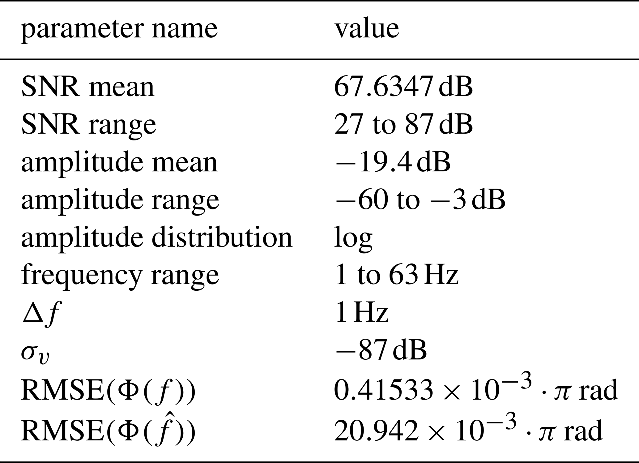
With the parameters listed in Table 1 random signals for testing are created according to the following equations:

$$\begin{array}{}\text{(44)}& {\displaystyle }{x}_{\mathrm{1}}(n,\mathit{\xi })=a_{\mathrm{1}}\left(\mathit{\xi }\right)\cdot \cos \left(\mathrm{2}\mathit{\pi }{\displaystyle \frac{f_{\mathrm{c}}\left(\mathit{\xi }\right)-\mathrm{0.5}\mathrm{\Delta }f\left(\mathit{\xi }\right)}{F_{\mathrm{s}}}}\cdot n+{\mathrm{\Phi }}_{\mathrm{1}}\left(\mathit{\xi }\right)\right)\text{(45)}& {\displaystyle }{x}_{\mathrm{2}}(n,\mathit{\xi })=a_{\mathrm{2}}\left(\mathit{\xi }\right)\cdot \cos \left(\mathrm{2}\mathit{\pi }{\displaystyle \frac{f_{\mathrm{c}}\left(\mathit{\xi }\right)+\mathrm{0.5}\mathrm{\Delta }f\left(\mathit{\xi }\right)}{F_{\mathrm{s}}}}\cdot n+{\mathrm{\Phi }}_{\mathrm{2}}\left(\mathit{\xi }\right)\right)\text{(46)}& {\displaystyle }y(n,\mathit{\xi })=x_{\mathrm{2}}(n,\mathit{\xi })+x_{\mathrm{2}}(n,\mathit{\xi })+v(n,\mathit{\xi })\end{array}$$

Figures 1 and 2 display one of the signals, that are generated with the described parameters. The time domain depiction shows both the generated and the reconstructed signals using the measured phase and amplitude. The displayed error

$$\begin{array}{}\text{(47)}& e_y\left(n\right)=y\left(n\right)-\widehat{x}\left(n\right)\end{array}$$

represents the difference between the measured signal

$$y\left(n\right)=x_{\mathrm{1}}\left(n\right)+x_{\mathrm{2}}\left(n\right)+v\left(n\right)$$

and the reconstructed signal:

$$\widehat{x}\left(n\right)={\widehat{x}}_{\mathrm{1}}\left(n\right)+{\widehat{x}}_{\mathrm{2}}\left(n\right)$$

The errors e_x1 and e_x2 are generated accordingly. The frequency domain representation displayed in Fig. 2 shows, that the measurement error e_y(n) approximates the actual measurement noise v(n) closely. Furthermore the power leakage from the windowed signals across the frequency spectrum is removed almost entirely. Due to the nature of the least squares algorithm used to derive the complex signal amplitudes, the residual PSD will be close to the sampling noise even with bad frequency estimates.

For further understanding of the limitations connected to the provided method of phase determination first some limitations of the ESPRIT algorithm are presented in Sect. 3.1 representative for a method of frequency estimation. In Sect. 3.2 the results are further investigated in regard to the resulting root mean square error (RMSE).

3.1 Limits of ESPRIT

When analyzing the resulting measurements, the limits ESPRIT must be examined. For this purpose a range of randomly distributed signals according to Table 1 is generated and analyzed using ESPRIT. Afterwards the measured oscillations corresponding to distinct signal frequencies are considered valid measurements. The ratio of correctly detected oscillations is displayed in Fig. 3.

Figure 3 Rate of successful signal separation based on ESPRIT: The number of successfully detected distinct oscillations in relation to the total number of measurements $r=N_{\mathrm{separated}}/N_{\mathrm{total}}$.

As shown in Fig. 3 the rate of correctly detected oscillation frequencies is mostly depending on the frequency separation Δf and the signal to noise ratio (SNR) of the sampled signal. Center frequency, input phase and power difference between both oscillations play a minor role.

Notable is the increase of erroneous detections close to 0 Hz and close to the Nyquist frequency 64 Hz. Below the minimum frequency of 1 Hz and above of 1 Hz below the Nyquist frequency the rate of correctly identified frequencies drops to less than 0.5. With a frequency separation above 0.14 Hz two oscillations can be separated in with a ratio above 0.5. At 0.32 Hz frequency separation this ratio becomes greater than 0.9. Applied to a radar system with a bandwidth of 250 MHz, as it is common in 24 GHz radar applications, this could result in a 90 % peak separation rate for reflecting surfaces with a distance of approximately 20 cm.

3.2 Measurement error analysis

The set of successfully separated signals is evaluated further. The system's accuracy is analyzed regarding the accuracy in frequency estimation and phase measurement. Table 2 gives a summarized overview of the performed signal simulation.

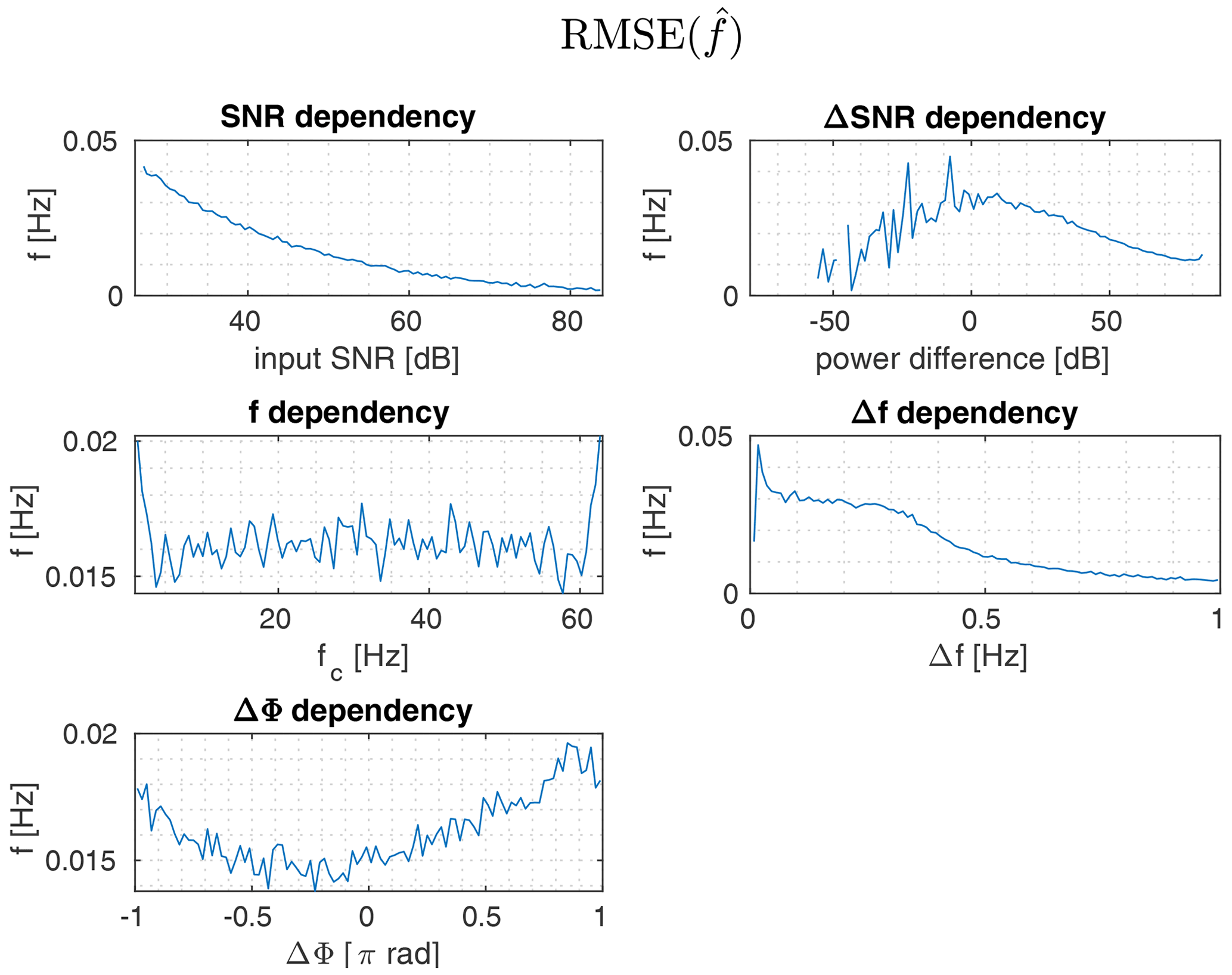
Figure 4 RMSE of the signal frequencies estimated by the ESPRIT method for all successfully separated signals.

Table 2 Summarized results.

The distribution of the estimated frequencies root mean square error (RMSE) displayed in Fig. 4 gives further insight into the performance of the utilized ESPRIT algorithm. The observed estimation error of the signal frequency is consistent with the results of successful frequency separation discussed in Sect. 3.1.

The resulting RMSE of the measured signal phase based on the actual signal frequencies is displayed in Fig. 5. The phase error distribution is comparable to the frequency error distribution, though the displayed results must be taken with a grain of salt, because measurements without successful frequency separation are excluded from the statistical RMSE analysis. This especially becomes clear when looking at the f and Δf subplots: In the upper and lower ranges of the center frequency f_c and below a frequency separation of Δf=0.4 Hz the phase error decreases. This is due to measurements with bad signal separation being disregarded. In general the phase estimation error is dependent primarily on the signal's SNR and decreases with increasing SNR and frequency separation.

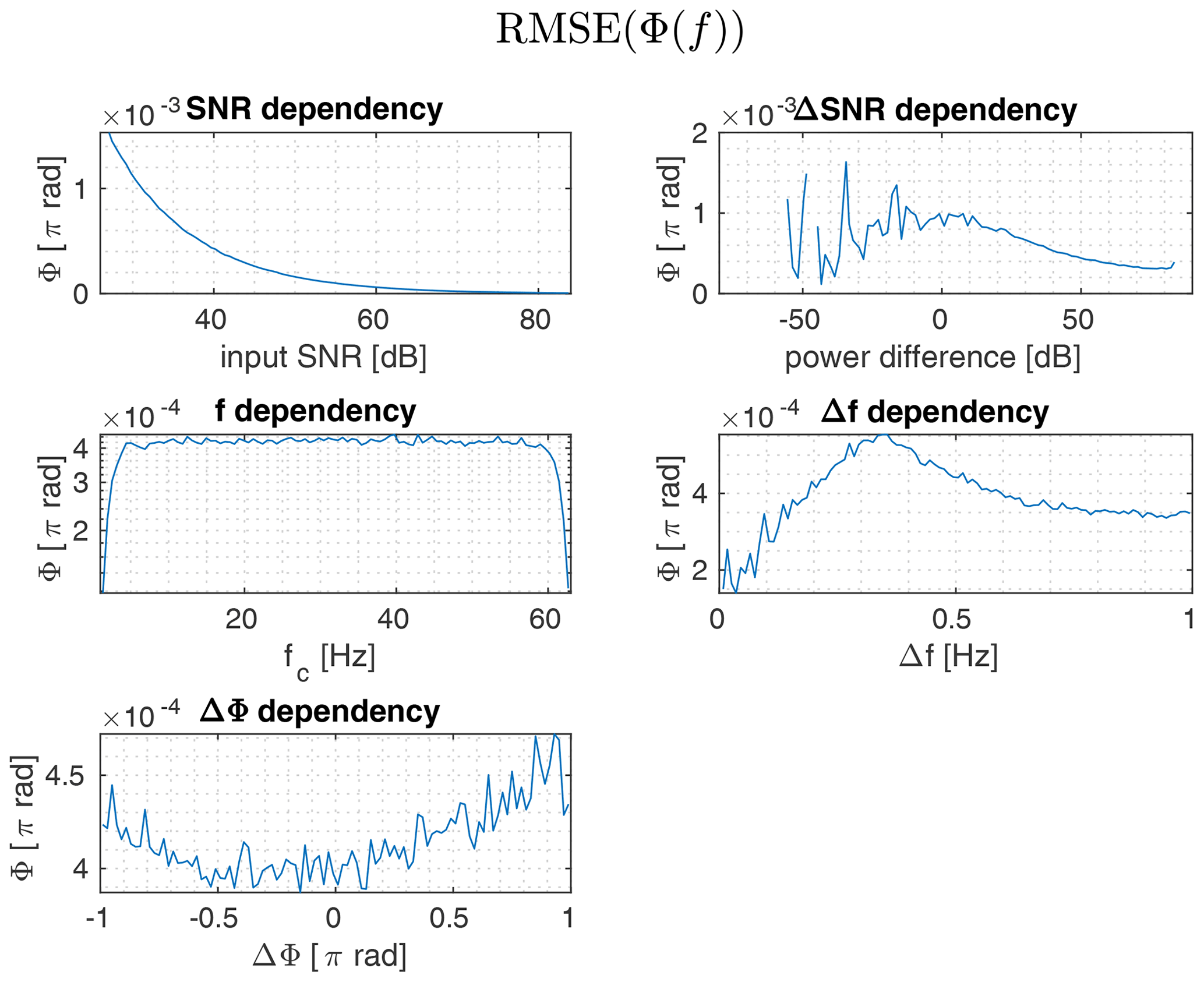
Figure 5 RMSE of the signal phase derived from the measured signal using the true signal frequency for the successfully separated signals.

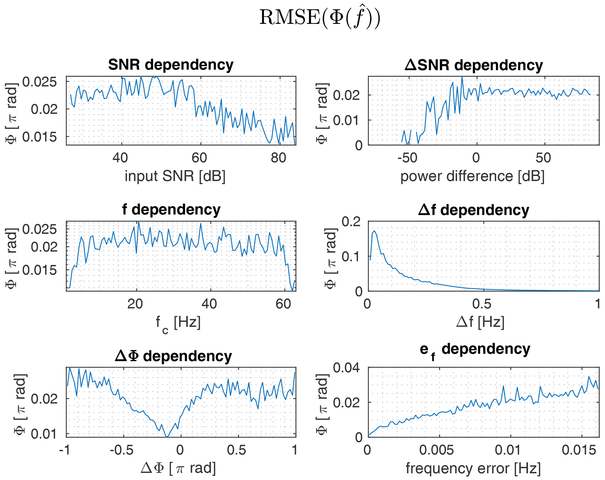
Figure 6 RMSE of the signal phase derived from the measured signal using the signal frequency estimated by the ESPRIT method for the successfully separated signals.

In comparison to the phase measurement based on the true frequency value, the phase error is two orders of magnitude worse, when it's based on imperfect frequency measurements. Across the complete set of measurements the root mean square error is 0.021π rad = 3.78^∘. Transferred to a 24 GHz radar application with a wavelength of 12 mm this transfers to a relative distance error of 63 µm. While the dependency on the signal to noise ratio (SNR) is almost negligible, the dependency on the frequency separation Δf becomes more obvious. As expected, an error in the estimated frequency results in an increased phase error.

4 Conclusions

In conclusion the method described in Sect. 2.3 represents a useful addition to frequency estimations like MUSIC or ESPRIT. While depending on the quality of the underlying frequency estimation, a very promising level of accuracy in phase measurement can be reached. Given that the analysis in this paper are done purely on synthetic data, further investigations using real world data are required.