Yield Optimization using Hybrid Gaussian Process Regression and a Genetic Multi-Objective Approach

Quantification and minimization of uncertainty is an important task in the design of electromagnetic devices, which comes with high computational effort. We propose a hybrid approach combining the reliability and accuracy of a Monte Carlo analysis with the efficiency of a surrogate model based on Gaussian Process Regression. We present two optimization approaches. An adaptive Newton-MC to reduce the impact of uncertainty and a genetic multi-objective approach to optimize performance and robustness at the same time. For a dielectrical waveguide, used as a benchmark problem, the proposed methods outperform classic approaches.

1 Introduction

In the manufacturing process of electromagnetic devices, e.g. antennas or filters, uncertainties may lead to deviations in the design parameters, e.g. geometry or material parameters. This may lead to rejections due to malfunctioning. Therefore, it is of great interest to estimate the impact of the uncertainty before production is started, and to minimize it if necessary in the design process.

The yield is a measure for the impact of uncertainty, it is defined as the fraction of realizations in a manufacturing process fulfilling some defined requirements, the so-called performance feature specifications (cf. Graeb, 2007). The relation between the yield Y and the failure probability F is given by $Y=\mathrm{1}-F$. A well established method for estimating the yield is Monte Carlo (MC) analysis (Hammersley and Handscomb, 1964, chap. 5). In a MC yield analysis, a large number of sample points is generated according to a given probability distribution of the uncertain design parameters. Then, the percentage of accepted sample points leads to the yield estimator. In order to decide if a sample point is accepted, a quantity of interest (QoI) has to be evaluated in order to check the performance feature specifications. In case of electrical engineering, very often this requires to solve partial differential equations originating from Maxwell's equations using the finite element method (FEM) for example. This implies high computational effort (cf. Hess and Benner, 2013).

There are two common approaches to improve the efficiency of MC analysis: reducing the number of sample points and reducing the computational effort for each evaluation of a sample point. Methods with regards to the first idea – reducing the number of sample points – are for example Importance Sampling (cf. Gallimard, 2019), or Subset Simulation (cf. Kouassi et al., 2016; Bect et al., 2017). In order to reduce the computational effort per evaluation, model order reduction (cf. Hess and Benner, 2013), or surrogate based approaches are used. Surrogate models are approximations (also known as response surfaces) of the original high fidelity model, which can be evaluated cheaply. Common surrogate model techniques are stochastic collocation (cf. Babuška et al., 2007) linear regression (cf. Rao and Toutenburg, 1999) Gaussian Process Regression (GPR) (cf. Rasmussen and Williams, 2006), and recently neural networks (cf. Goodfellow et al., 2016). The two approaches for efficiency improvement can also be combined, e.g., Tyagi et al. (2018) use Importance Sampling and GPR.

This work deals with the efficient estimation of the yield using a hybrid approach combining the efficiency of a surrogate model approach and the accuracy and reliability of a classic MC analysis (cf. Li and Xiu, 2010; Tyagi et al., 2018). The surrogate model is based on GPR, which has the feature that the model can be easily updated during the estimation process (see Fuhrländer and Schöps, 2020). The optimization algorithm maximizing the yield is based on a globalized Newton method (Ulbrich and Ulbrich, 2012, chap. 10.3). The presented method is similar to the adaptive Newton-MC method in Fuhrländer et al. (2020), but GPR is used here for the surrogate model instead of stochastic collocation. Due to the blackbox character of GPR, the opportunity arises to use this algorithm in combination with commercial FEM software. Finally, we formulate a new optimization problem and propose a genetic multi-objective optimization (MOO) approach in order to maximize robustness, i.e., the yield, and performance simultaneously.

2 Definition of the yield

Let p be the vector of uncertain design parameters. They are modeled as random variables with a joint probability density function denoted by pdf(p). Following Graeb (2007) the performance feature specifications are defined as inequalities in terms of one (or more) QoIs Q, which have to be fulfilled for all so-called range parameter values r, e.g. frequencies, within a certain interval T_r, i.e.,

$$\begin{array}{}\text{(1)}& Q_r\left(\mathit{p}\right)\le c\forall r\in T_r.\end{array}$$

Without loss of generality the performance feature specifications are defined as one upper bound with a constant c∈ℝ. The safe domain is the set of all design parameters, for which the performance feature specifications are fulfilled, i.e.,

$${\mathrm{\Omega }}_{\text{s}}:=\left\{\mathit{p}\left|Q_r\right(\mathit{p})\le c\forall r\in T_r\right\}.$$

Then, the yield is introduced as (Graeb, 2007, chap. 4.8.3, Eq. 137)

$$\begin{array}{}\text{(2)}& Y\left(\stackrel{\mathrm{‾}}{\mathit{p}}\right):=\mathbb{E}\left[{\mathbf{1}}_{{\mathrm{\Omega }}_{\text{s}}}\left(\mathit{p}\right)\right]:=\underset{-\mathrm{\infty }}{\overset{\mathrm{\infty }}{\int }}\mathrm{\dots }\underset{-\mathrm{\infty }}{\overset{\mathrm{\infty }}{\int }}{\mathbf{1}}_{{\mathrm{\Omega }}_{\text{s}}}\left(\mathit{p}\right)\text{pdf}\left(\mathit{p}\right)\text{d}\mathit{p},\end{array}$$

where 𝔼 is the expected value and ${\mathbf{1}}_{{\mathrm{\Omega }}_{\text{s}}}\left(\mathit{p}\right)$ the indicator function which has value 1 if p lies in Ω_s and 0 otherwise.

For yield estimation and the proposed genetic MOO approach, there are no restrictions on the distribution of the random inputs. For the single-objective optimization approach based on the Newton method, the gradient and the Hessian of the yield need to be calculated. For Gaussian distributed random inputs, an analytical formulation is known (see Sect. 4), for other distributions a difference quotient can be used (with additional computing effort) or a non-gradient based optimizer can be employed. In the following, we assume that the uncertain design parameters are truncated Gaussian distributed (cf. Cohen, 2016) i.e., $\mathit{p}\sim {\mathcal{N}}_{\mathcal{T}}(\stackrel{\mathrm{‾}}{\mathit{p}},\mathbf{\Sigma },\mathit{l}\mathit{b},\mathit{u}\mathit{b})$, where $\stackrel{\mathrm{‾}}{\mathit{p}}$ denotes the mean value, Σ the covariance matrix and $\mathit{l}\mathit{b}=\stackrel{\mathrm{‾}}{\mathit{p}}-\mathrm{\Delta }\mathit{p}$ and $\mathit{u}\mathit{b}=\stackrel{\mathrm{‾}}{\mathit{p}}+\mathrm{\Delta }\mathit{p}$ the lower and upper bounds, where Δp is a vector with positive entries. The covariance matrix originates from the given uncertainties in the manufacturing process and is assumed to be unchangeable. With the intention of highlighting the dependence of the truncated Gaussian distributed probability density function on $\stackrel{\mathrm{‾}}{\mathit{p}}$, Σ, lb and ub we write ${\text{pdf}}_{{\mathcal{N}}_{\mathcal{T}}(\stackrel{\mathrm{‾}}{\mathit{p}},\mathbf{\Sigma },\mathit{l}\mathit{b},\mathit{u}\mathit{b})}\left(\mathit{p}\right)$.

3 Yield estimation

A classic MC analysis would consist in generating a set of N_MC sample points and calculating the fraction of sample points p_i lying inside the safe domain. The MC yield estimator is then given by (Hammersley and Handscomb, 1964, chap. 5)

$${\stackrel{\mathrm{̃}}{Y}}_{\text{MC}}\left(\stackrel{\mathrm{‾}}{\mathit{p}}\right)={\displaystyle \frac{\mathrm{1}}{N_{\text{MC}}}}\sum _{i=\mathrm{1}}^{N_{\text{MC}}}{\mathbf{1}}_{{\mathrm{\Omega }}_{\text{s}}}\left({\mathit{p}}_i\right).$$

A commonly used error indicator for the MC analysis is

$$\begin{array}{}\text{(3)}& {\mathit{\sigma }}_{{\stackrel{\mathrm{̃}}{Y}}_{\text{MC}}}=\sqrt{{\displaystyle \frac{{\stackrel{\mathrm{̃}}{Y}}_{\text{MC}}\left(\stackrel{\mathrm{‾}}{\mathit{p}}\right)\left(\mathrm{1}-{\stackrel{\mathrm{̃}}{Y}}_{\text{MC}}\left(\stackrel{\mathrm{‾}}{\mathit{p}}\right)\right)}{N_{\text{MC}}}}}\le {\displaystyle \frac{\mathrm{0.5}}{\sqrt{N_{\text{MC}}}}},\end{array}$$

where ${\mathit{\sigma }}_{\stackrel{\mathrm{̃}}{Y}}$ is the standard deviation of the yield estimator (cf. Giles, 2015). Thus, for high accuracy a large sample size is needed, which means high computational effort, i.e., note the square root in the denominator.

In this work, we focus on surrogate based approaches. These approaches are common in order to reduce the computational effort of MC analysis, by reducing the computational effort of each model evaluation. Nevertheless, one has to be careful when replacing a model by a surrogate for MC analysis. In most surrogate approaches, e.g. stochastic collocation, the computational effort to build the surrogate model increases rapidly with an increasing number of uncertain parameters (curse of dimensionality; cf. Bellman, 1961). And, in Li and Xiu (2010) it is shown, that there are examples, where the yield estimator fails drastically, even though the surrogate model seems highly accurate. Therefore, Li and Xiu (2010) introduce a hybrid approach. Its basic idea is to distinguish between critical sample points and non-critical sample points. Critical sample points are those which are close to the border between safe domain and failure domain, see the red sample points in Fig. 1 (left) for a visualization with two uncertain parameters. While most of the sample points are only evaluated on a surrogate model, the critical sample points are also evaluated on the original model. Only then it is decided if the sample point is accepted or not. By this strategy, accuracy and reliability can be maintained while computational effort can be reduced. A crucial point is the definition of the critical sample points, i.e., of the term close to the border.

Figure 1 Critical (red) and non-critical (green) sample points.

The hybrid approach we use in this work is based on Li and Xiu (2010) and is explained more detailed in Fuhrländer and Schöps (2020). As surrogate model we use GPR, i.e., we approximate the QoI as Gaussian Process (GP) and assume that the error of the surrogate model is Gaussian distributed. For detailed information about GPR we refer to Rasmussen and Williams (2006, chap. 2). One advantage of GPR is that the standard deviation σ(p_i) of the GP may serve as an error indicator of the surrogate model and thus can be used to find the critical sample points. With GPR predictor $\stackrel{\mathrm{̃}}{Q}\left({\mathit{p}}_i\right)$ and safety factor γ>1 we define a sample point p_i as critical, if

$${\stackrel{\mathrm{̃}}{Q}}_{r_j}\left({\mathit{p}}_i\right)-\mathit{\gamma }{\mathit{\sigma }}_{r_j}\left({\mathit{p}}_i\right)<c<{\stackrel{\mathrm{̃}}{Q}}_{r_j}\left({\mathit{p}}_i\right)+\mathit{\gamma }{\mathit{\sigma }}_{r_j}\left({\mathit{p}}_i\right)$$

holds for any r_j, where r_j is a discretization of T_r with $j=\mathrm{1},\mathrm{\dots },N_{\text{range}}$. In this case, $Q_{r_j}\left({\mathit{p}}_i\right)$ is evaluated on the original model, before classifying p_i as accepted or not accepted, see the red case in Fig. 1 (right, γ=2). Using another surrogate technique, e.g. stochastic collocation, would require commonly the calculation of a separate error indicator, e.g. with adjoint methods (cf. Fuhrländer et al., 2020). This requires additional computing time and in case of adjoint error indicators, knowledge about the system matrices, which is not always given when using proprietary FEM implementations. After classifying the sample points, the GPR-Hybrid yield estimator is calculated by

$${\stackrel{\mathrm{̃}}{Y}}_{\text{GPR-H}}\left(\stackrel{\mathrm{‾}}{\mathit{p}}\right)={\displaystyle \frac{\mathrm{1}}{N_{\text{MC}}}}\left(\sum _{\begin{array}{c}{\mathit{p}}_i\\ \text{crit.}\end{array}}{\mathbf{1}}_{{\mathrm{\Omega }}_{\text{s}}}\left({\mathit{p}}_i\right)+\sum _{\begin{array}{c}{\mathit{p}}_j\\ \text{non-crit.}\end{array}}{\mathbf{1}}_{{\stackrel{\mathrm{̃}}{\mathrm{\Omega }}}_{\text{s}}}\left({\mathit{p}}_j\right)\right),$$

where ${\stackrel{\mathrm{̃}}{\mathrm{\Omega }}}_{\text{s}}$ is the safe domain based on the performance feature specifications with the approximated QoI.

Figure 2 Flowchart for the Hybrid-GPR approach.

Another advantage of GPR is that we are not limited to specific training data, e.g. points on a tensor grid as in polynomial approaches (e.g. the stochastic collocation approach in Fuhrländer et al., 2020), and thus we can add arbitrary points in order to update the GPR model on the fly. This allows us to start with a rather small initial training data set and improve the GPR model during the estimation by adding the critical sample points to the training data set without much extra cost. Also, sorting the sample points before classification can increase the efficiency (cf. Bect et al., 2012). For more details and possible modifications of the estimation with the GPR-Hybrid approach, we refer to Fuhrländer and Schöps (2020). The flowchart in Fig. 2 shows the basic procedure of the Hybrid-GPR approach for yield estimation.

4 Yield optimization

After estimating the impact of uncertainty, often a minimization of this impact is desired. In the following we propose two optimization approaches. In the first approach, we assume that a performance optimization was carried out in a previous step, and focus here on the maximization of the yield. The optimization problem reads

$$\begin{array}{}\text{(4)}& \underset{\stackrel{\mathrm{‾}}{\mathit{p}}}{max}Y\left(\stackrel{\mathrm{‾}}{\mathit{p}}\right)\stackrel{\left(\mathrm{2}\right)}{=}\underset{\stackrel{\mathrm{‾}}{\mathit{p}}}{max}\underset{-\mathrm{\infty }}{\overset{\mathrm{\infty }}{\int }}\mathrm{\dots }\underset{-\mathrm{\infty }}{\overset{\mathrm{\infty }}{\int }}{\mathbf{1}}_{{\mathrm{\Omega }}_{\text{s}}}\left(\mathit{p}\right){\text{pdf}}_{{\mathcal{N}}_{\mathcal{T}}(\stackrel{\mathrm{‾}}{\mathit{p}},\mathbf{\Sigma },\mathit{l}\mathit{b},\mathit{u}\mathit{b})}\left(\mathit{p}\right)\text{d}\mathit{p}.\end{array}$$

Please note that we model this optimization problem as unconstrained, since the performance feature specifications (1) are considered within the indicator function, i.e., within the safe domain Ω_s. However, it is also possible to include constraints and use another optimization method. Further, note that the optimization variable $\stackrel{\mathrm{‾}}{\mathit{p}}$ appears only in the probability density function. Thus, when calculating the gradient with respect to $\stackrel{\mathrm{‾}}{\mathit{p}}$ for optimization purpose, only the derivative of the probability density function needs to be calculated, see Graeb (2007, chap. 7.1), i.e.,

$${\mathrm{\nabla }}_{\stackrel{\mathrm{‾}}{\mathit{p}}}Y\left(\stackrel{\mathrm{‾}}{\mathit{p}}\right)=\underset{-\mathrm{\infty }}{\overset{\mathrm{\infty }}{\int }}\mathrm{\dots }\underset{-\mathrm{\infty }}{\overset{\mathrm{\infty }}{\int }}{\mathbf{1}}_{{\mathrm{\Omega }}_{\text{s}}}\left(\mathit{p}\right){\mathrm{\nabla }}_{\stackrel{\mathrm{‾}}{\mathit{p}}}{\text{pdf}}_{{\mathcal{N}}_{\mathcal{T}}\left(\stackrel{\mathrm{‾}}{\mathit{p}},\mathbf{\Sigma },\mathit{l}\mathit{b},\mathit{u}\mathit{b}\right)}\left(\mathit{p}\right)\text{d}\mathit{p}.$$

For a Gaussian distribution the probability density function is an exponential function, thus the gradient (and the Hessian, respectively) can be calculated analytically. This would allow us an efficient use of a gradient based algorithm like a globalized Newton method (Ulbrich and Ulbrich, 2012, chap. 10.3). For that reason we use the probability density function of a Gaussian distribution ${\text{pdf}}_{\mathcal{N}(\stackrel{\mathrm{‾}}{\mathit{p}},\mathbf{\Sigma })}$ instead of ${\text{pdf}}_{{\mathcal{N}}_{\mathcal{T}}(\stackrel{\mathrm{‾}}{\mathit{p}},\mathbf{\Sigma },\mathit{l}\mathit{b},\mathit{u}\mathit{b})}$ in order to calculate the derivatives for the Newton method. Using a Gaussian distribution instead of a truncated Gaussian distribution can be understood as applying an inexact Newton method (cf. Dembo et al., 1982). In Fuhrländer et al. (2020), the difference between the analytical inexact gradient (of the Gaussian distribution) and the difference quotient gradient (of the truncated Gaussian distribution) and its effect on the optimization procedure has been investigated. The results justify the assumption of the use of an inexact Newton method. For other distributions, e.g. uniform distributions, a difference quotient can be used instead of the analytical gradient and Hessian.

From Eq. (3) we know that the size of the sample set is crucial for the accuracy of the yield estimator, but it is also crucial for the efficiency of the algorithm. Typically, in the first steps of the Newton method high accuracy of the yield estimator is not necessary as long as the gradient indicates an ascent direction. Thus, we modify the Newton algorithm from Ulbrich and Ulbrich (2012) and propose an adaptive Newton-MC method, where we start with a small sample size $N_{\text{MC}}^{\text{start}}$. When the solution shows no improvement and the target accuracy ${\widehat{\mathit{\sigma }}}_{{\stackrel{\mathrm{̃}}{Y}}_{\text{GPR-H}}}$ is not reached in the kth step, i.e.,

$$\left|{\stackrel{\mathrm{̃}}{Y}}_{\text{GPR-H}}\left({\stackrel{\mathrm{‾}}{\mathit{p}}}^{k-\mathrm{1}}\right)-{\stackrel{\mathrm{̃}}{Y}}_{\text{GPR-H}}\left({\stackrel{\mathrm{‾}}{\mathit{p}}}^k\right)\right|<{\widehat{\mathit{\sigma }}}_{{\stackrel{\mathrm{̃}}{Y}}_{\text{GPR-H}}}$$

and

$${\displaystyle \frac{\mathrm{1}}{\mathrm{2}}}{\widehat{\mathit{\sigma }}}_{{\stackrel{\mathrm{̃}}{Y}}_{\text{GPR-H}}}<{\mathit{\sigma }}_{{\stackrel{\mathrm{̃}}{Y}}_{\text{GPR-H}}\left({\stackrel{\mathrm{‾}}{\mathit{p}}}^k\right)},$$

then the sample size is increased to $N_{\text{MC}}^k=N_{\text{MC}}^k+N_{\text{MC}}^{\text{start}}$. The detailed procedure can be found in Fuhrländer et al. (2020). As a novelty, here, the GPR-Hybrid approach is used for yield estimation.

In the second approach, we formulate a multi-objective optimization problem to optimize yield and performance at the same time. Without loss of generality it can be formulated as

$$\begin{array}{}\text{(5)}& \underset{\stackrel{\mathrm{‾}}{\mathit{p}}}{min}{f}_m\left(\stackrel{\mathrm{‾}}{\mathit{p}}\right),m=\mathrm{1},\mathrm{\dots },M\end{array}$$

$$\begin{array}{lll}\text{s.t. }& g_n\left(\stackrel{\mathrm{‾}}{\mathit{p}}\right)\le \mathrm{0},& n=\mathrm{1},\mathrm{\dots },N\\ & {\stackrel{\mathrm{‾}}{p}}_i^{\mathit{l}\mathit{b}}\le {\stackrel{\mathrm{‾}}{p}}_i\le {\stackrel{\mathrm{‾}}{p}}_i^{\mathit{u}\mathit{b}},& i=\mathrm{1},\mathrm{\dots },\text{dim}\left(\stackrel{\mathrm{‾}}{\mathit{p}}\right),\end{array}$$

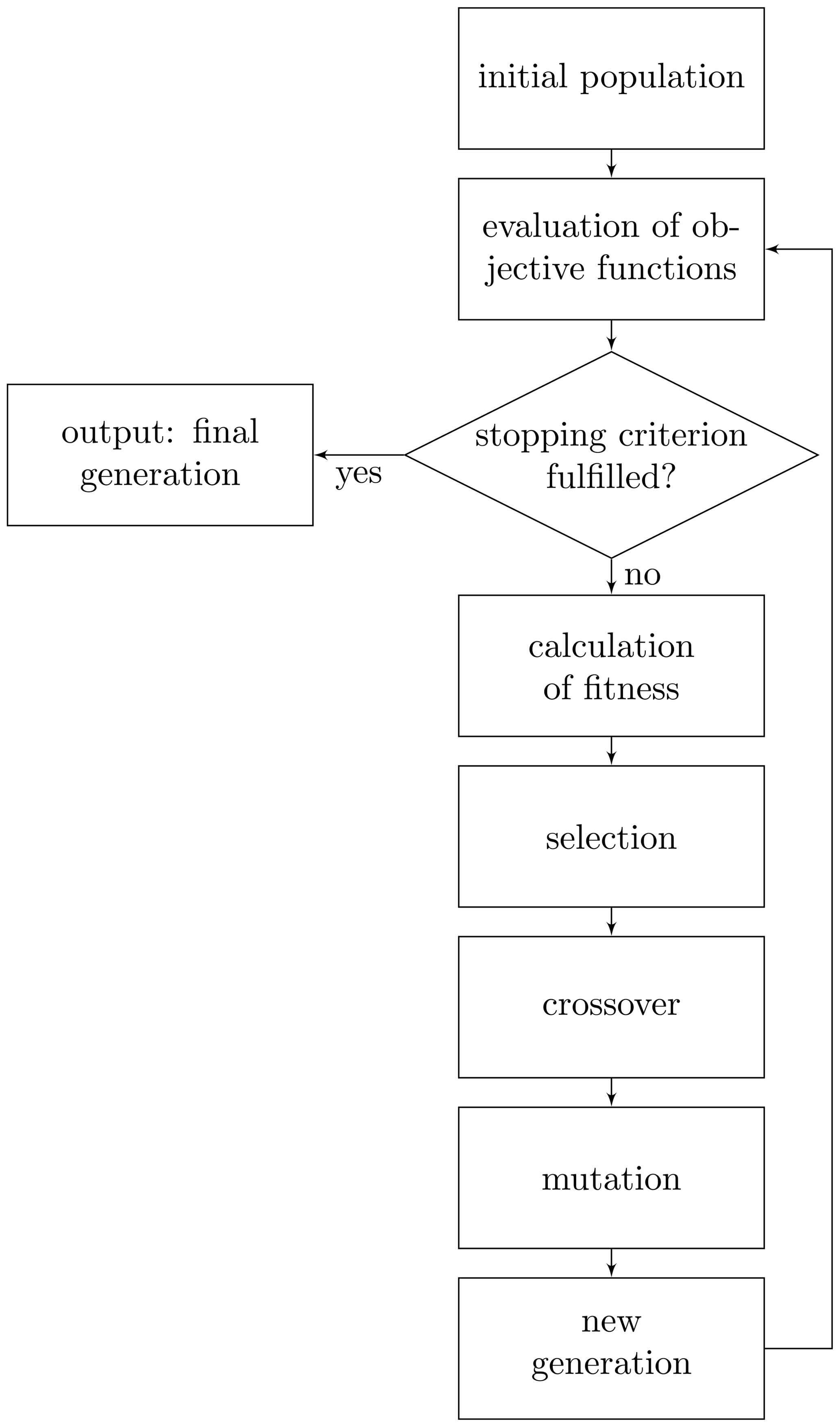
with $f_{\mathrm{1}}\left(\stackrel{\mathrm{‾}}{\mathit{p}}\right)=-Y\left(\stackrel{\mathrm{‾}}{\mathit{p}}\right)$ and $f_m\left(\stackrel{\mathrm{‾}}{\mathit{p}}\right)$, $m=\mathrm{2},\mathrm{\dots },M$ are key performance indicators, e.g. cost or performance functions. By solving this optimization problem, we aim to obtain the pareto front, which is the set of pareto optimal solutions (Ehrgott, 2005, Def. 2.1). For any pareto optimal solution holds, that one objective value can only be improved at the cost of another objective value. Classic approaches include the weighted sum or the ε-constraint method (Ehrgott, 2005, chaps. 3–4). However, these methods require convexity of the pareto front, which cannot be guaranteed in this context. Furthermore, they always find only one pareto optimal solution for each run of the solver, thus they need to be solved many times with different settings in order to approximate the entire pareto front. Genetic algorithms, however, approximate the entire pareto front in one run. But for this purpose, a swarm of solutions needs to be evaluated. Thus, genetic algorithms are also computationally expensive. In genetic algorithms an initial population of individuals is generated, in our case the individuals are randomly generated $\stackrel{\mathrm{‾}}{\mathit{p}}$-values. For each individual, all objective functions from Eq. (5) are evaluated. This information is used to calculate the so-called fitness of a solution. Based on the fitness value, promising individuals of the initial population are selected (selection rule). These individuals are recombined (crossover rule) in order to create new individuals, the so-called offsprings. These offsprings are manipulated, often with a certain probability (mutation rule). From parts of the individuals of the initial population and the offsprings, a new generation is created. This procedure is repeated until some stopping criterion is reached, e.g. number of generations or improvement in the solution or objective space. The output is a generation of individuals approximating the pareto front. A simplified visualization of the procedure is shown in Fig. 3. For more details about genetic algorithms we refer to Audet and Hare (2017). In contrast to the above mentioned classic methods, genetic algorithms do not require convexity or any other previous knowledge about the problem.

Figure 3 Flowchart for the genetic MOO approach.

5 Numerical results

We apply the proposed methods for yield estimation and yield optimization to a benchmark problem in the context of electromagnetic field simulations. The benchmark problem is a rectangular waveguide with dielectrical inlay, see Fig. 4. In the following we briefly describe the model of the waveguide, for more details we refer to Fuhrländer et al. (2020) and Loukrezis (2019). From the time harmonic Maxwell's formulation on the domain D⊆ℝ³ we derive the curl-curl equation of the E-field formulation

$$\mathrm{\nabla }\times \left({\mathit{\mu }}^{-\mathrm{1}}\mathrm{\nabla }\times {\mathbf{E}}_{\mathit{\omega }}\right)-{\mathit{\omega }}^{\mathrm{2}}\mathit{\epsilon }{\mathbf{E}}_{\mathit{\omega }}=\mathrm{0}\text{on }D.$$

It is to be solved for the electric field phasor E_ω, where ω denotes the angular frequency, μ the permeability and ε the permittivity. Discretizing the weak formulation by (high order) Nédélec basis functions leads to an approximated E-field ${\stackrel{\mathrm{̃}}{\mathbf{E}}}_{\mathit{\omega }}$. Let ${\mathrm{\Gamma }}_{{\text{P}}_{\mathrm{1}}}$ and ${\mathrm{\Gamma }}_{{\text{P}}_{\mathrm{2}}}$ denote the two ports of the waveguide. We assume that the waveguide is excited at port ${\mathrm{\Gamma }}_{{\text{P}}_{\mathrm{1}}}$ by an incident TE₁₀ wave. Then, the QoI is the FEM approximation of the scattering parameter (S-parameter) of the TE₁₀ mode on ${\mathrm{\Gamma }}_{{\text{P}}_{\mathrm{1}}}$. We write

$$\begin{array}{}\text{(6)}& Q_{\mathit{\omega }}\left(\mathit{p}\right)=q\left({\stackrel{\mathrm{̃}}{\mathbf{E}}}_{\mathit{\omega }}\left(\mathit{p}\right)\right).\end{array}$$

Figure 4 FEM model of a rectangular waveguide with dielectrical inlay.

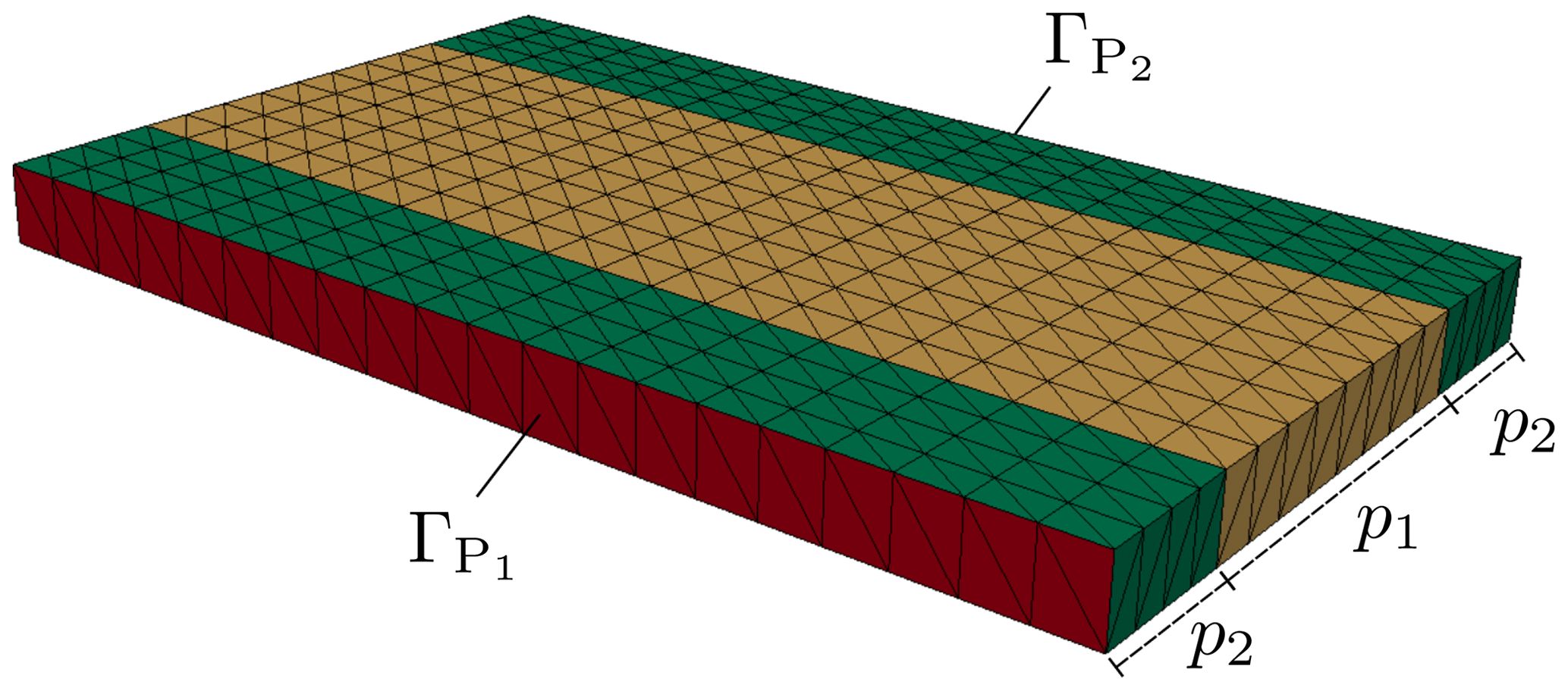
For uncertainty quantification we consider the waveguide with four uncertain parameters: two geometrical parameters p₁ (length of the inlay in mm) and p₂ (length of the offset in mm) and two material parameters p₃ and p₄, with the following impact on the relative permeability and permittivity of the inlay:

$$\begin{array}{c}{\displaystyle }{\mathit{ϵ}}_r=\mathrm{1}+p_{\mathrm{3}}+\left(\mathrm{1}-p_{\mathrm{3}}\right){\left(\mathrm{1}+j\mathit{\omega }{\left(\mathrm{2}\mathit{\pi }\mathrm{5}\times {\mathrm{10}}^{\mathrm{9}}\right)}^{-\mathrm{1}}\right)}^{-\mathrm{1}},\\ {\displaystyle }{\mathit{\mu }}_r=\mathrm{1}+p_{\mathrm{4}}+\left(\mathrm{2}-p_{\mathrm{4}}\right){\left(\mathrm{1}+j\mathit{\omega }{\left(\mathrm{1.1}\cdot \mathrm{2}\mathit{\pi }\mathrm{20}\times {\mathrm{10}}^{\mathrm{9}}\right)}^{-\mathrm{1}}\right)}^{-\mathrm{1}}.\end{array}$$

For the generation of the MC sample we assume the uncertain parameters to be truncated Gaussian distributed. The mean and the covariance matrix are given by

$$\begin{array}{c}{\displaystyle }\stackrel{\mathrm{‾}}{\mathit{p}}=[\mathrm{10.36},\mathrm{4.76},\mathrm{0.58},\mathrm{0.64}{]}^{\text{T}},\\ {\displaystyle }\mathbf{\Sigma }=\text{diag}\left(\left[{\mathrm{0.7}}^{\mathrm{2}},{\mathrm{0.7}}^{\mathrm{2}},{\mathrm{0.3}}^{\mathrm{2}},{\mathrm{0.3}}^{\mathrm{2}}\right]\right).\end{array}$$

The geometrical parameters are truncated at ±3 mm and the material parameters at ±0.3. By this truncation, we avoid the generation of unphysical values (e.g. negative distances). With the frequency as range parameter the performance feature specifications are

$$\begin{array}{}\text{(7)}& Q_{\mathit{\omega }}\left(\mathit{p}\right)\le -\mathrm{24}\text{dB}\end{array}$$

with ω=2πf $\forall f\in T_f=\left[\mathrm{6.5},\mathrm{7.5}\right]$ in GHz. The frequency range T_f is parametrized in 11 equidistant frequency points. Then, a sample point is accepted, if the inequality in Eq. (7) holds for all frequency points in the discretized range parameter interval T_d⊂T_f.

For the estimation we set an initial training data set of 10 sample points and an allowed standard deviation of the yield ${\widehat{\mathit{\sigma }}}_{{\stackrel{\mathrm{̃}}{Y}}_{\text{GPR-H}}}\le \mathrm{0.01}$ which leads to a sample size of N_MC=2500, cf. Eq. (3). In order to build the GPR surrogate the python package scikit-learn is used (cf. Pedregosa et al., 2011). For each frequency point, a separate GPR model is built for the real part and the imaginary part. For the GP we use the mean value of the training data evaluations as mean function and the squared exponential kernel

$$k\left(\mathit{p},{\mathit{p}}^{\prime }\right)=\mathit{\zeta }{\text{e}}^{-\frac{{\left|\mathit{p}-{\mathit{p}}^{\prime }\right|}^{\mathrm{2}}}{\mathrm{2}{l}^{\mathrm{2}}}}.$$

The two hyperparameters ζ∈ℝ and l>0 are internally optimized within the scikit-learn package. For GPR the default settings of scikit-learn have been used, except for the following modifications: the starting value for ζ has been set to 0.1, its optimization bounds to $\left[{\mathrm{10}}^{-\mathrm{5}},{\mathrm{10}}^{-\mathrm{1}}\right]$ and the noise factor $\mathit{\alpha }={\mathrm{10}}^{-\mathrm{5}}$.

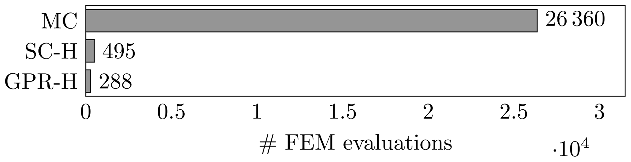
We compare the proposed GPR-Hybrid approach with the hybrid approach based on stochastic collocation (SC-Hybrid) from Fuhrländer et al. (2020), but without adaptive mesh refinement. As reference solution we consider the classic MC analysis. Both hybrid methods achieve the same accuracy, i.e., the same yield estimator as the MC reference, ${\stackrel{\mathrm{̃}}{Y}}_{\text{MC}}\left(\stackrel{\mathrm{‾}}{\mathit{p}}\right)=\mathrm{95.44}$ %. In order to compare the computational effort we consider the number of FEM evaluations, necessary for solving Eq. (6). In all methods a short circuit strategy has been used such that a sample point is not evaluated on a frequency point if it has already been rejected for another frequency point. Figure 5 shows the comparison of these methods. The lower number of FEM evaluations in the GPR-Hybrid approach compared to SC-Hybrid can be explained by the fact that the surrogate model can be updated on the fly.

Figure 5 Computational effort for yield estimation.

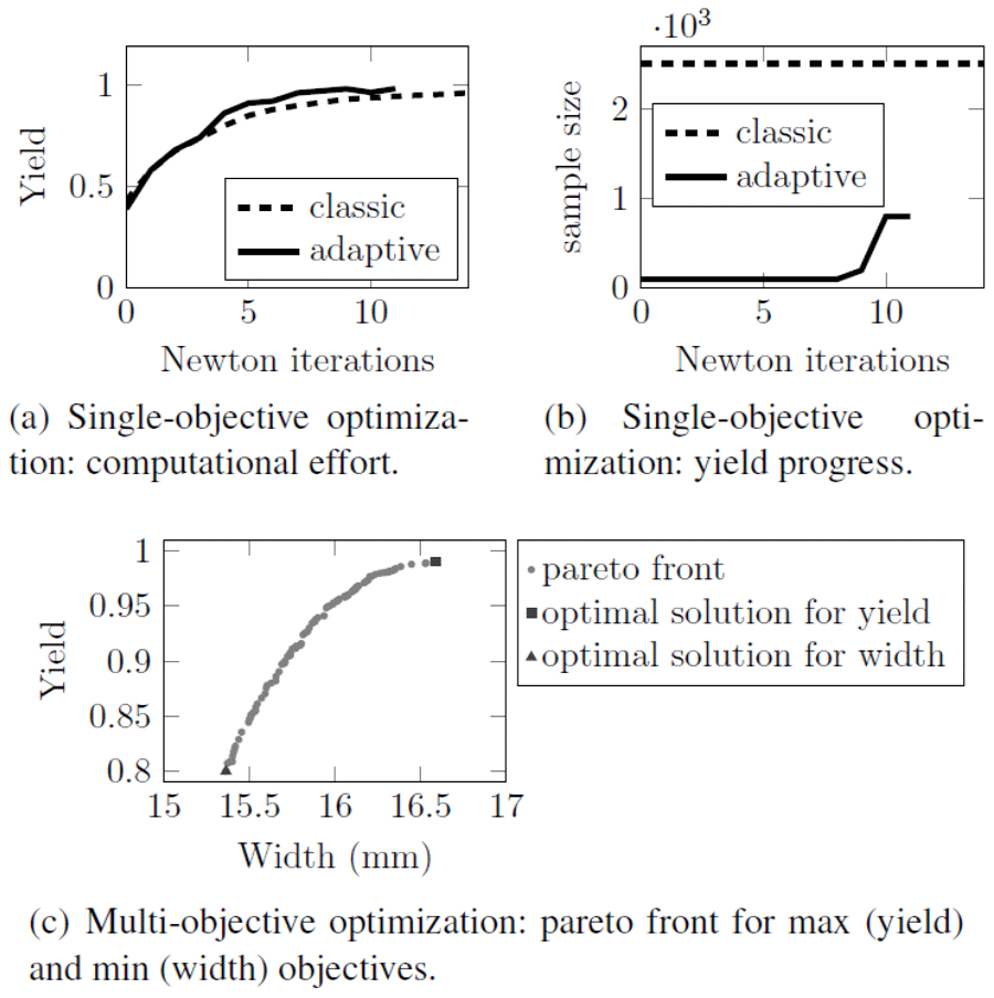
For the single-objective optimization in Eq. (4) we use the same settings as above and additionally the starting point ${\stackrel{\mathrm{‾}}{\mathit{p}}}^{\mathrm{0}}=[\mathrm{9},\mathrm{5},\mathrm{1},\mathrm{1}{]}^{\text{T}}$ and the initial sampling size $N_{\text{MC}}^{\text{start}}=\mathrm{100}$ in the adaptive method. Figure 6a and b show the increase of the yield and the sample size in each iteration for the adaptive Newton-MC compared with a classic Newton method with a fixed sample size. Both methods achieve the same optimal yield of ${\stackrel{\mathrm{̃}}{Y}}_{\text{GPR-H}}\left({\stackrel{\mathrm{‾}}{\mathit{p}}}^{\text{opt}}\right)=\mathrm{98.32}$ %. The adaptive Newton-MC needs 11 iterations and 571 FEM evaluations for that, the classic Newton method 37 iterations and 2643 FEM evaluations.

Figure 6 Single- and multi-objective optimization.

For the multi-objective optimization in Eq. (5) the python package pymoo has been used (cf. Blank and Deb, 2020). We formulate a second objective function to minimize the expected width of the waveguide. Further we request the yield to be larger than a minimal value Y_min=0.8, include this as a constraint and define lower and upper bounds for the mean value of the uncertain parameter. We obtain the optimization problem

$$\begin{array}{c}{\displaystyle }\underset{\stackrel{\mathrm{‾}}{\mathit{p}}}{min}\left(-Y\left(\stackrel{\mathrm{‾}}{\mathit{p}}\right)\right)\\ {\displaystyle }\underset{\stackrel{\mathrm{‾}}{\mathit{p}}}{min}{\mathbb{E}}_{{\mathcal{N}}_{\mathcal{T}}}\left[p_{\mathrm{1}}+\mathrm{2}{p}_{\mathrm{2}}\right]\end{array}$$

$${\displaystyle }\begin{array}{ll}\text{s.t. }& g_{\mathrm{1}}\left(\stackrel{\mathrm{‾}}{\mathit{p}}\right)=Y_{\text{min}}-Y\left(\stackrel{\mathrm{‾}}{\mathit{p}}\right)\le \mathrm{0},\\ & {\left[\mathrm{5},\mathrm{3},\mathrm{0.5},\mathrm{0.5}\right]}^{\text{T}}\le \stackrel{\mathrm{‾}}{\mathit{p}}\le {\left[\mathrm{25},\mathrm{15},\mathrm{1.5},\mathrm{1.5}\right]}^{\text{T}},\end{array}$$

where ${\mathbb{E}}_{{\mathcal{N}}_{\mathcal{T}}}\equiv {\mathbb{E}}_{{\text{pdf}}_{{\mathcal{N}}_{\mathcal{T}}(\stackrel{\mathrm{‾}}{\mathit{p}},\mathbf{\Sigma },\mathit{l}\mathit{b},\mathit{u}\mathit{b})}}$ denotes the expected value with respect to the distribution of the uncertain parameter p. In pymoo, the NSGA2 solver and the default settings have been used, except for the following modifications: initial population size was set to 200, number of offsprings per generation to 100 and maximum number of generations to 30. In Fig. 6c we see the pareto front after 30 generations. Depending on the rating of the significance of the two objective functions, a solution can be chosen.

6 Conclusions

Reliable and efficient methods for yield estimation and optimization have been presented. The hybrid approach based on a GPR surrogate model including opportunity to model updates reduces the computational effort significantly, while maintaining high accuracy. The proposed adaptive Newton-MC reduces the uncertainty impact with low cost compared to classic Newton methods. A new multi-objective approach allows optimizing performance and robustness simultaneously. In future, we will work on improving the efficiency of multi-objective optimization based on genetic algorithms by using adaptive sample size increase and GPR approximations of the yield, in addition to the GPR approximations of the QoIs.