 | 21 Mar 2023
Migrating and nonmigrating tidal signatures in sporadic E layer occurrence rates
Kanykei Kandieva
Christina Arras
We analyse sporadic E (ES) layer occurrence rates (OR) obtained from ionospheric GPS radio occultation measurements by the FORMOSAT-3/COSMIC constellation. Maximum OR are seen at 95–105 km altitude. Midlatitude ES layers are mainly due to wind shear in the presence of tides, and the strongest signals are the migrating diurnal and semidiurnal components. Especially in the Southern Hemisphere, nonmigrating components such as a diurnal westward wave 2 and a semidiurnal westward wave 1 are also visible, especially at higher latitudes. Near the equator, a strong diurnal eastward wavenumber 3 component and a semidiurnal eastward wavenumber 2 component occur in summer and autumn. Terdiurnal and quarterdiurnal components are weaker than the diurnal and semidiurnal ones.
- Article
(3783 KB) - Full-text XML
- BibTeX
- EndNote


Sporadic E (ES) layers are thin regions of accumulated ions in the lower ionosphere. At midlatitudes, they are most frequently found during the summer season (e.g., Arras et al., 2008). ES layers are generally formed at heights between 90 and 120 km. Their occurrence can be described through the wind shear theory (Whitehead, 1961; Yamazaki et al., 2022), which includes the interaction between the Earth's magnetic field, the vertical shear of the neutral wind, and the metallic ion concentration (e.g., Fytterer et al., 2014; Gong et al., 2014).
The dynamics of the lower thermosphere at time scales up to one day are mainly influenced by solar tides, having periods of a solar day and its harmonics (e.g., Forbes, 1995). Tidal amplitudes usually are maximum around or above 120 km, where they are of the order of magnitude of the mean wind, or even larger. Tidal waves of shorter periods often have smaller amplitudes, so that, on average, the major diurnal variability of lower thermosphere winds is due to the diurnal tide (DT, Pancheva et al., 2002; Wu et al., 2008) and the semidiurnal tide (SDT, Pancheva et al., 2002; Wu et al., 2011; Pokhotelov et al., 2018). Note that, however, at higher midlatitudes the DT wind amplitudes become small compared with SDT ones during most of the year. To a lesser degree, also to the terdiurnal tide (TDT, Beldon et al., 2006; Liu et al., 2019) contributes to lower thermospheric wind variability. Owing to its smaller amplitude, the quarterdiurnal tide (QDT) has been analysed less frequently in the past, but more recently the QDT has attained increasing attention (Liu et al., 2015; Azeem et al., 2016; Jacobi et al., 2017, 2019; Guharay et al., 2018).
Solar tides are a major source of vertical wind shear, and the tidal contribution to the overall wind shear is frequently larger than the one of the background wind. Therefore, tide-like structures are also expected in ES layer occurrence rates (OR). Consequently, tides are generally accepted to be the major driver of midlatitude ES (Mathews, 1998), and they lead to the downward moving tidal signatures in ionosonde registrations (e.g., Haldoupis et al., 2006; Haldoupis, 2012). However, ES parameters can be modulated by planetary waves (e.g., Karami et al., 2012), and this may lead to variations of the central period of ES variations (Koucká Knížová et al., 2021). Analysing ES layer OR observed by GPS together with meteor radar wind measurements at Collm (51.3∘ N, 13.0∘ E), a clear correspondence of ES layer OR and negative wind shear maximums has been found for the SDT (Arras et al., 2009), TDT (Fytterer et al., 2013), and QDT (Jacobi et al., 2019), but not for the DT (Jacobi and Arras, 2019). Liu et al. (2018) found that the global distribution of ES layers is relatively consistent with the wind shear distribution. Fytterer et al. (2014) and Jacobi et al. (2019) compared GPS radio occultation (RO) observations of ES layer OR and modelled wind shear. They demonstrated the similarity of the TDT and QDT in ES OR and wind shear on a global scale. Resende et al. (2018a) modelled the connection of ES layers and tides, although focusing on the equatorial region, where electric field effects become more important than at middle latitudes.
Comparisons of ES layers and wind shear have frequently been performed based on local wind measurements (Arras et al., 2009; Fytterer et al., 2013; Jacobi et al., 2019; Jacobi and Arras, 2019). These observations cannot distinguish between migrating and nonmigrating tidal components. To reveal the migrating ES tidal components only, these results were compared with ES OR sampled in local time at all longitudes. This approach showed good correspondence for Northern Hemisphere (NH) midlatitude stations, where the migrating tidal component is obviously dominating.
Using frequency-wavenumber analysis, it is possible to analyse also nonmigrating tidal components from global fields. Therefore, in the following, we present analyses of migrating but also nonmigrating tidal signatures seen in ES layer OR, which are based on FORMOSAT-3/COSMIC GPS RO observations. We will use the following notation: The period is represented by the letter D, S, T, Q for diurnal, semidiurnal, terdiurnal, and quarterdiurnal, respectively. This is followed by W or E for westward or eastward, and an integer representing the zonal wavenumber. Thus, DW1 represents the diurnal westward migrating tide of zonal wavenumber 1, SE2 stands for the semidiurnal eastward wavenumber 2 component, and so forth.
Note that the correspondence between the wind shear and the ES layer OR diurnal variability is much weaker for the DT than for the SDT, TDT, and QDT. This is owing to the fact that a diurnal ES layer variation is not only due to wind shear, but also owing to background ionization, which is much stronger during daytime. Strictly speaking, it is therefore incorrect to interpret the diurnal ES layer variation as a DT signature. For a consistent description, we nevertheless refer to the diurnal ES layer signature as a DT.
We make use of ionospheric RO measurements (UCAR, 2022) by the FORMOSAT-3/COSMIC constellation, which performed observations in both the neutral and ionized atmosphere (Anthes et al., 2008), making use of a constellation of six low-Earth orbiting (LEO) satellites. During each occultation, signals of the rising or setting GPS satellites are received by a LEO satellite. When the signals pass the atmosphere and ionosphere of the Earth, they are influenced by atmospheric properties. This is in particular true for the ionospheric electron density, which causes refraction and degradation of the GPS waves. This effect can be utilized to obtain information about the ionosphere and its disturbances. Observation of the neutral atmosphere is also possible, but this is out of the scope of this study. Detailed information on the RO technique principles can be found in Hajj et al. (2002) and Kursinski et al. (1997).
In this study the Signal-to-Noise Ratio (SNR) profiles of the GPS L1 phase measurements (using the atmPhs data product) are analysed according to Arras and Wickert (2018). The SNR is very sensitive to vertical variations of the electron density, and these occur particularly within an ES layer. These vertically localized electron density variations lead to phase fluctuations of the GPS signal, which can be observed as changes in the received signal strength (Hajj et al., 2002). In order to avoid unwanted influences from the different basic signal power values on the further data analysis, every SNR profile is normalized first. In the case of the absence of ionospheric disturbances, the SNR value is almost constant at altitudes above about 35 km. The SNR standard deviation is calculated in 2.5 km altitude intervals. The SNR profile is considered to be disturbed when it exceeds an empirically found threshold of 0.2. If large standard deviation values are concentrated within a thin layer of less than 10 km vertical extent, we assume that the respective SNR profile includes the signature of an ES layer. The height where the SNR value deviates most from the mean of the SNR profile is considered as the altitude of the ES layer. This has been validated by comparisons with ionosonde ES layer observations (Arras and Wickert, 2018; Resende et al., 2018b).
The following analysis is based on observations from 2007 to 2017. The number of occultations and the number of observed ES layers are each binned into a 4-dimensional grid of (latitude × longitude × altitude × time), calculated within partly overlapping boxes of 10∘ (latitude), 20∘ (longitude), 10 km (altitude) and 1 h, respectively, and as 3-monthly (seasonal) means. ES OR are then calculated as the number of ES layers divided by the number of occultations in each bin. Note that the OR of an individual bin is set to zero if there are less than five occultations within this bin.
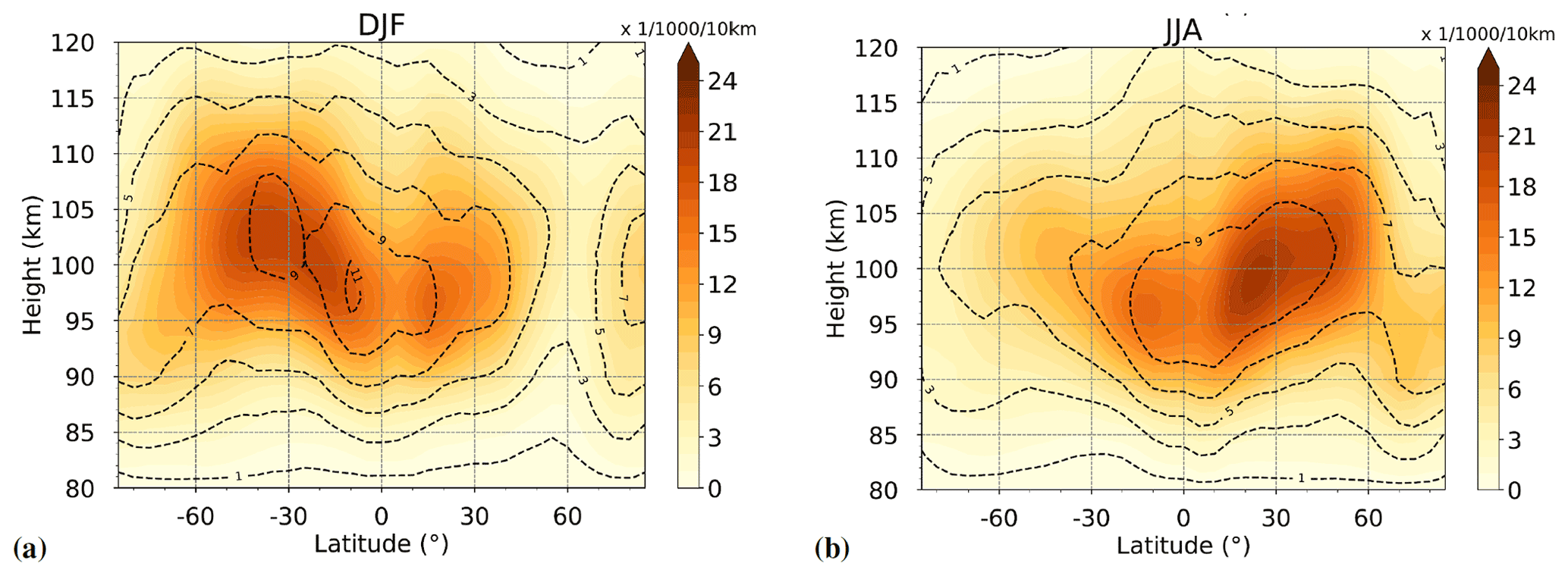
Figure 1Zonal and seasonal mean ES layer occurrence rates in a 10 km vertical window each for (a) DJF, (b) JJA. Data are averages over 2007–2017. Dashed lines show standard deviations.
Figure 1 shows the 2007–2017 mean zonal mean and seasonal mean ES layer OR for December–February (DJF), and June–August (JJA) together with their standard deviations calculated from the respective data of each year. The distributions are similar to those shown, e.g., by Fytterer et al. (2014) or Jacobi et al. (2019) obtained from a more limited dataset. Maximum OR are found at altitudes between 95 and 105 km. OR maximize in summer, which is thought to be owing to increased meteor influx during that season (Haldoupis et al., 2007). The summer maximum is more pronounced in the NH, which is due to the weaker magnetic field within the South Atlantic Anomaly (e.g., Arras et al., 2008; Chu et al., 2014; Arras and Wickert, 2018). Near the equator, ES layer OR are small, owing to the horizontal magnetic field at the magnetic equator, which does not allow the electrons to follow the vertically moving ions (e.g., Abdu et al., 1996; Arras et al., 2008, 2010; Arras and Wickert, 2018).
In order to analyse the tidal components in the long-term diurnal ES signal, we performed frequency-wavenumber (f–k) analyses that are based on gridded data that again have been sampled in boxes of in latitude and longitude, resp., and 10 km in height. Here, we analyse results in windows centered at 100 km. We present results for four seasons, namely winter (DJF), spring (March–May, MAM), summer (JJA) and autumn (September–November, SON).
Note that the amplitudes of OR oscillations, or tidal components in OR, are determined by the tidal activity and its corresponding wind shear, but also by the background ionization of metallic ions. The latter in particular produces a DW1 signature, but this is not connected with wind shear, as can be seen, e.g., in phase comparisons shown by Jacobi et al. (2019). Furthermore, the seasonal cycle and global structure of ES OR amplitudes also reflect the respective background OR, which is, among others, determined by the meteor influx (Haldoupis et al., 2007; Jacobi et al., 2013). Removing the background variability by normalizing OR amplitudes by the OR background (e.g., Fytterer et al., 2014; Jacobi et al., 2019) usually leads to a stronger correspondence of the wind shear and ES amplitude distributions. Therefore, in the following we use relative amplitudes (RA), defined as the OR amplitudes divided by the background OR.
4.1 Diurnal and semidiurnal components
The latitudinal distributions of DT RA spectra are shown in Fig. 2 for different seasons. Only RA exceeding three times their standard error are presented. Clearly, the migrating DW1 dominates in all seasons and at all latitudes except for the Southern Hemisphere (SH) summer. Maximum values are seen at midlatitudes in contrast to neutral wind amplitudes (Stober et al., 2021), and this may be explained by the fact the diurnal ES layer OR not necessarily show a tidal signature, but rather are owing to the background diurnal ionisation (see, e.g., Jacobi et al., 2019). Neutral atmosphere wind DW1 maximize at lower latitudes equatorward of 30∘ (Wu et al., 2008). In Fig. 2, maximum ES amplitudes are partly seen at higher latitudes, again indicating a weak correlation with the wind shear.
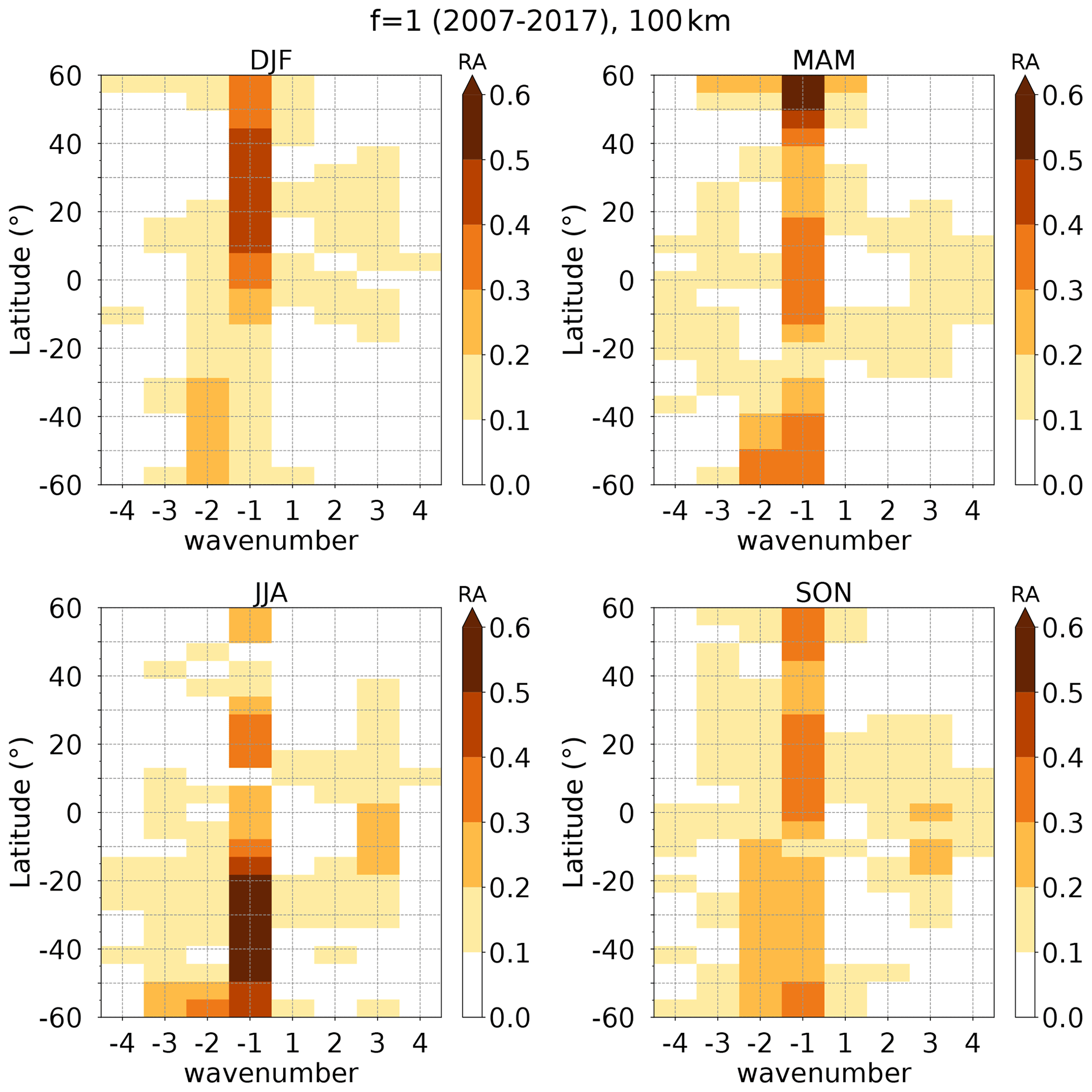
Figure 2Latitudinal distribution of DT wavenumber spectra of relative ES OR RA in the 95–105 km height window.
Particularly in the SH, there is also a DW2 component, with a tendency for greater amplitudes at higher latitudes. Indications for a DW2 component in satellite observations of neutral winds have been presented by Manson et al. (2004). At the equator and at low SH latitudes, a DE3 is visible in the NH summer and autumn. The DE3 signature has been observed in several atmospheric (e.g., Manson et al., 2004) and ionospheric parameters (Pancheva and Mukhtarov, 2010, 2012), and a DE3 in ES layer occurrence has recently been presented by Liu et al. (2021). Pancheva and Mukhtarov (2010) also reported the existence of a DE2 in ionospheric heights and neutral temperatures, however, the DE2 is only weakly visible in ES layer OR here (Fig. 2). Note that there is a strong migrating DW1 signature at higher latitudes especially during equinox months, which is not connected with tidal activity, but is probably due to the action of magnetospheric electric fields (Kirkwood and Nilsson, 2000). Electric fields force ion convergence leading to ES layer formation at polar latitudes. The polar electric fields vary during the course of the day causing a diurnal signature in ES layers formed by them.
The SDT (Fig. 3), as is the case with the DT, is mainly due to the migrating SW2, although nonmigrating components are visible as well, and they are somewhat more pronounced than for the DT. The SDT amplitudes are largest at middle and particularly higher latitudes, but lower at low latitudes. This corresponds to results from satellite observations of the SDT in neutral winds (Burrage et al., 1995; Wu et al., 2011). However, at higher NH latitudes, the SDT amplitudes maximise in spring and summer, while neutral wind amplitudes are largest in autumn and winter (e.g., Pokhotelov et al., 2018). Near the equator, the SDT is larger again, with a dominant migrating SW2, and eastward components visible especially in NH summer and autumn. At middle latitudes, and partly at equatorial latitudes, a SW3 is also visible, with a tendency of being more expressed in the SH than in the NH. The SW3 has also been observed in satellite wind analyses (Manson et al., 2004). At higher latitudes, a clear SW1 is also visible in all months, which is stronger in the SH than in the NH. According to Miyoshi et al. (2017), the SW3 and SW1 are excited by tropospheric heating during equinoxes, and during solstices they are generated in the winter stratosphere and mesosphere through the nonlinear interaction between the stationary planetary wave and the migrating SDT.
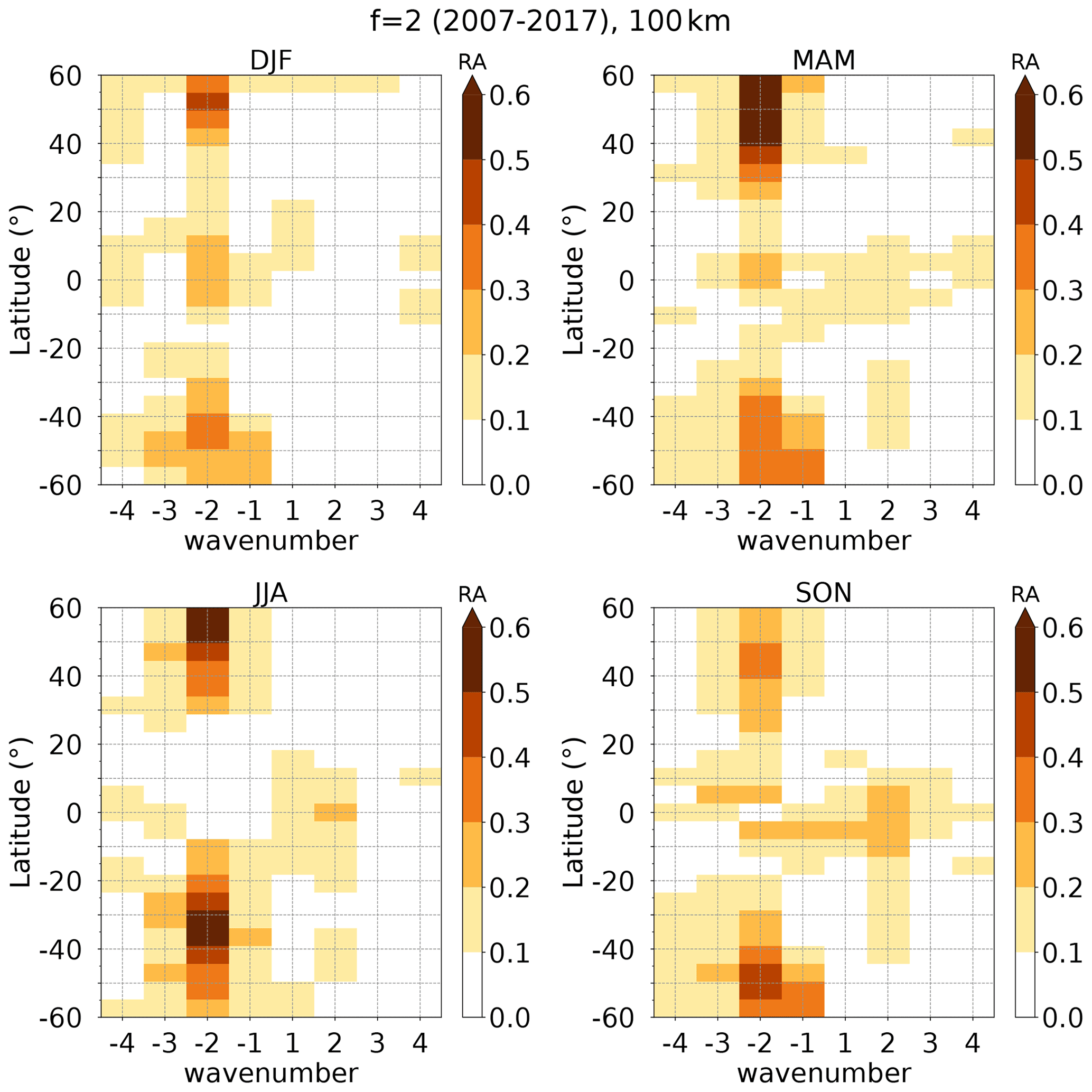
Near the equator, eastward propagating SDT components are visible, and the strongest of them is the SE2, occurring during each month, and maximising during NH summer and autumn. The SE2 tide is thought to be excited by latent heat release in the tropical troposphere and net radiative heating (Zhang et al., 2010). Pancheva and Mukhtarov (2012) showed the SE2 in COSMIC F2 region electron densities, but these maximised at middle latitudes (about 30∘) and not at the equator. Further nonmigrating SDT components, occurring mainly in autumn, are the SE1 and SW1 (Fig. 3).
A the equator, during late summer/autumn, the eastward propagating nonmigrating components, mainly the DE3 and the SE2, are dominating, and their amplitudes even exceed the ones of the migrating components then. This is shown in Fig. 4. While the migrating components do not show a very pronounced seasonal cycle at the equator, the DE3 and SE2 are small in NH winter, and maximise in late summer/early autumn.
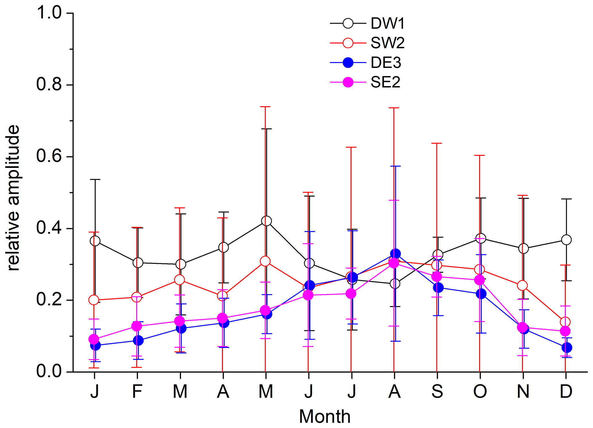
Figure 4Seasonal distribution of relative amplitudes of DE3 and SE2 in the 95–105 km height window at the equator, together with the respective migrating DW1 and SW2 amplitudes. Error bars show standard deviations.
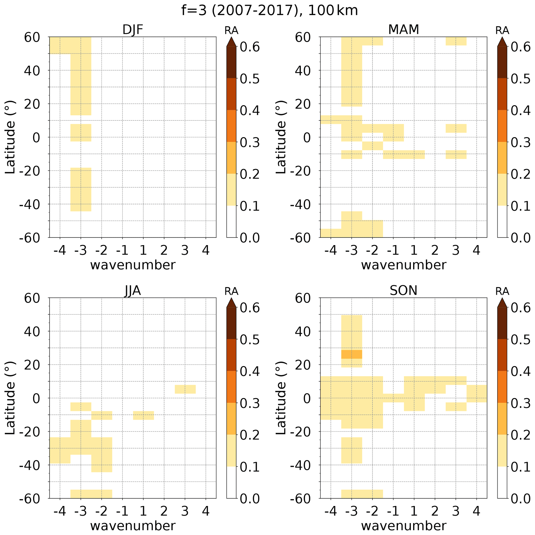
4.2 Terdiurnal and quarterdiurnal components
The latitudinal distributions of TDT components in ES layer RA are shown in Fig. 5. Their amplitudes are smaller than the semidiurnal and diurnal ones. The migrating TW3 is clearly visible and it is the dominating TDT component in ES layer OR. At NH midlatitudes, there is a tendency for larger TW3 values during winter and equinoxes, and for weaker values in summer. This is also the case for the neutral wind TDT (Beldon et al., 2006) and indicates a relation with neutral wind shear (Fytterer et al., 2014). There is a considerable activity of nonmigrating TDT components, in particular of a TW2. In some seasons and at especially at low latitudes in autumn, also a TW4, TW1, and some eastward propagating nonmigrating components are visible.
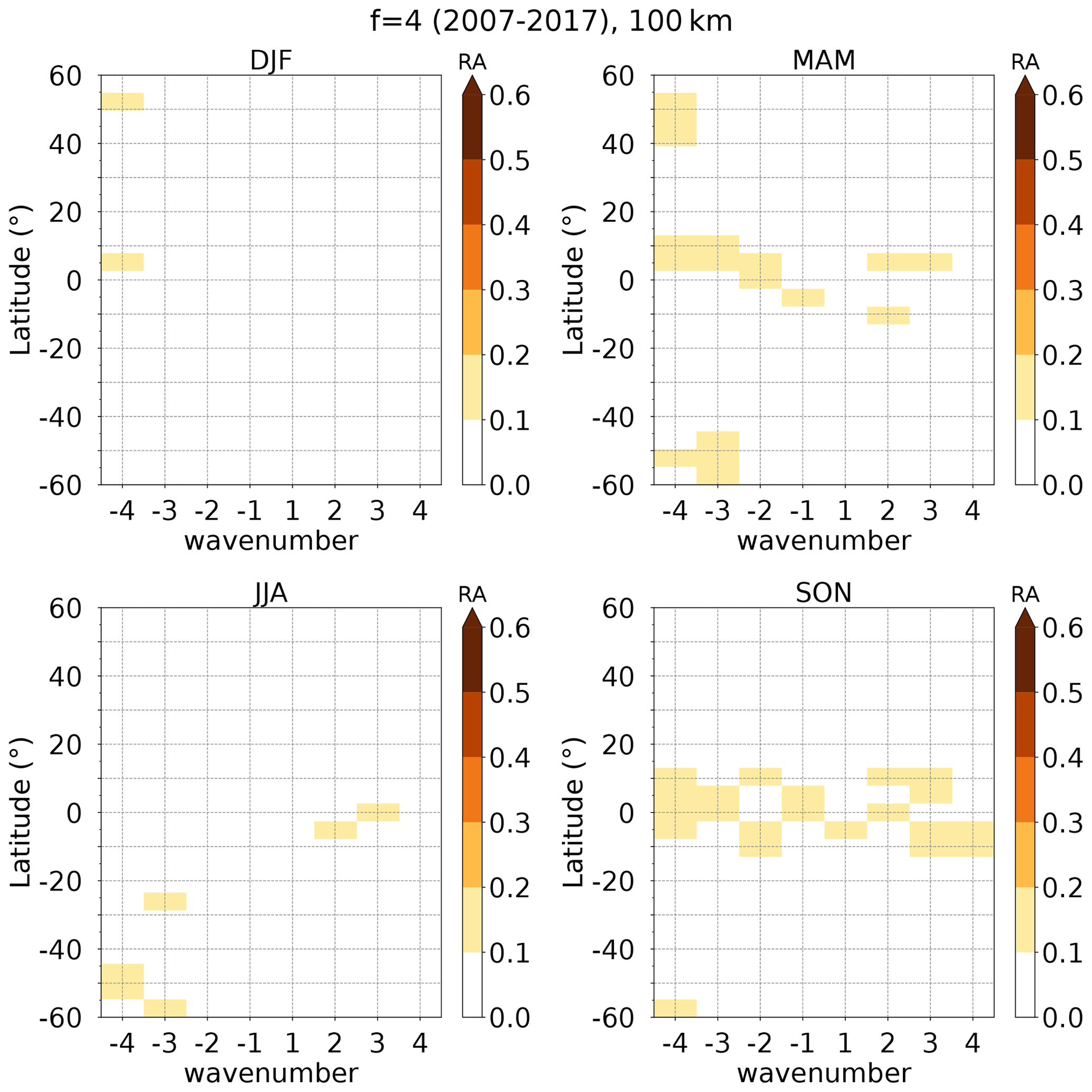
QDT components are shown in Fig. 6. Their amplitudes are much weaker than the DT, SDT, and also TDT ones. The QDT is more irregular than other components. The migrating QW4 does not obviously dominate in most months and at most latitudes. There are also indications for nonmigrating components, especially near the equator and during equinoxes. During summer, QDT activity at higher midlatitudes is barely visible and not significant. There is a tendency for slightly stronger QW4 activity during higher midlatitude winter and spring, which has been shown for the QW4 in winds and ES layer OR by Jacobi et al. (2017, 2019).
We analysed ES layer OR obtained from GPS RO measurements at lower ionospheric heights. Maximum OR are seen at 95–105 km altitude. The strongest tidal signals, as shown by their relative amplitudes RA are due to the migrating DW1 and SW2. Their global structure is partly similar to the one of neutral wind tides, but this is not the case for all components.
More strongly expressed in the SH than in the NH, nonmigrating components such as a DW2 and a SW1 are also visible, especially at higher latitudes. Near the equator, a clear DE3 and also a SE2 occur in summer and autumn, together with further eastward components. Terdiurnal and in particular quarterdiurnal components are weaker than the diurnal and semidiurnal ones.
Nonmigrating components such as SW1, SW3, and DW2 tend to be stronger in the SH than in the NH, at least for the DT and SDT components. This is probably due to the more non-zonal structure of the magnetic field and consequently the ES layer distribution, which minimizes at the South Atlantic Anomaly.
Radio occultation data are freely available from UCAR on https://data.cosmic.ucar.edu/gnss-ro/cosmic1/ (UCAR, 2022).
CJ initiated the study and prepared the first draft of the paper. KK performed the tidal analyses based on GPS ES OR, which had been provided by CA. All authors actively contributed to the writing of the final version.
The contact author has declared that neither they nor their co-authors have any competing interests.
Publisher's note: Copernicus Publications remains neutral with regard to jurisdictional claims in published maps and institutional affiliations.
This article is part of the special issue “Kleinheubacher Berichte 2021”.
The provision of FORMOSAT-3/COSMIC data by University Corporation for Atmospheric Research is gratefully acknowledged. We thank Friederike Lilienthal, Leipzig, for providing the first version of the f–k analyses software.
This research has been supported by the Deutsche Forschungsgemeinschaft (grant nos. JA 836/38-1 and AR953/1-2).
This paper was edited by Ralph Latteck and reviewed by Petra Koucka Knizova and one anonymous referee.
Abdu, M. A., Batista, I. S., Muralikrishna, P., and Sobral, J. H. A.: Long term trends in sporadic E layers and electric fields over Fortaleza, Brazil, Geophys. Res. Lett., 23, 757–760, https://doi.org/10.1029/96GL00589, 1996. a
Anthes, R. A., Bernhardt, P. A., Chen, Y., Cucurull, L., Dymond, K. F., Ector, D., Healy, S. B., Ho, S.-P., Hunt, D. C., Kuo, Y.-H., Liu, H., Manning, K., McCormick, C., Meehan, T. K., Randel, W. J., Rocken, C., Schreiner, W. S., Sokolovskiy, S. V., Syndergaard, S., Thompson, D. C., Trenberth, K. E., Wee, T.-K., Yen, N. L., and Zeng, Z.: The COSMIC/FORMOSAT-3 Mission: Early Results, B. Am. Meteorol. Soc., 89, 313–334, https://doi.org/10.1175/BAMS-89-3-313, 2008. a
Arras, C. and Wickert, J.: Estimation of ionospheric sporadic E intensities from GPS radio occultation measurements, J. Atmos. Sol.-Terr. Phys., 171, 60–63, https://doi.org/10.1016/j.jastp.2017.08.006, 2018. a, b, c, d
Arras, C., Wickert, J., Beyerle, G., Heise, S., Schmidt, T., and Jacobi, C.: A global climatology of ionospheric irregularities derived from GPS radio occultation, Geophys. Res. Lett., 35, L14809, https://doi.org/10.1029/2008GL034158, 2008. a, b, c
Arras, C., Jacobi, C., and Wickert, J.: Semidiurnal tidal signature in sporadic E occurrence rates derived from GPS radio occultation measurements at higher midlatitudes, Ann. Geophys., 27, 2555–2563, https://doi.org/10.5194/angeo-27-2555-2009, 2009. a, b
Arras, C., Jacobi, C., Wickert, J., Heise, S., and Schmidt, T.: Sporadic E signatures revealed from multi-satellite radio occultation measurements, Adv. Radio Sci., 8, 225–230, https://doi.org/10.5194/ars-8-225-2010, 2010. a
Azeem, I., Walterscheid, R. L., Crowley, G., Bishop, R. L., and Christensen, A. B.: Observations of the migrating semidiurnal and quaddiurnal tides from the RAIDS/NIRS instrument, J. Geophys. Res.-Space, 121, 4626–4637, https://doi.org/10.1002/2015JA022240, 2016. a
Beldon, C., Muller, H., and Mitchell, N.: The 8-hour tide in the mesosphere and lower thermosphere over the UK, 1988–2004, J. Atmos. Sol.-Terr. Phys., 68, 655–668, https://doi.org/10.1016/j.jastp.2005.10.004, 2006. a, b
Burrage, M. D., Hagan, M. E., Skinner, W. R., Wu, D. L., and Hays, P. B.: Long-term variability in the solar diurnal tide observed by HRDI and simulated by the GSWM, Geophys. Res. Lett., 22, 2641–2644, https://doi.org/10.1029/95GL02635, 1995. a
Chu, Y. H., Wang, C. Y., Wu, K. H., Chen, K. T., Tzeng, K. J., Su, C. L., Feng, W., and Plane, J. M. C.: Morphology of sporadic E layer retrieved from COSMIC GPS radio occultation measurements: Wind shear theory examination, J. Geophys. Res.-Space, 119, 2117–2136, https://doi.org/10.1002/2013JA019437, 2014. a
Forbes, J. M.: Tidal and Planetary Waves, AGU – American Geophysical Union, 67–87, https://doi.org/10.1029/GM087p0067, 1995. a
Fytterer, T., Arras, C., and Jacobi, C.: Terdiurnal signatures in sporadic E layers at midlatitudes, Adv. Radio Sci., 11, 333–339, https://doi.org/10.5194/ars-11-333-2013, 2013. a, b
Fytterer, T., Arras, C., Hoffmann, P., and Jacobi, C.: Global distribution of the migrating terdiurnal tide seen in sporadic E occurrence frequencies obtained from GPS radio occultations, Earth Planets Space, 66, 1–9, https://doi.org/10.1186/1880-5981-66-79, 2014. a, b, c, d, e
Gong, Y., Zhou, Q., and Zhang, S.: Numerical and observational study of ion layer formation at Arecibo, in: XXXIth URSI General Assembly, Beijing, China, 1–4, https://doi.org/10.1109/URSIGASS.2014.6929732, 2014. a
Guharay, A., Batista, P. P., Buriti, R. A., and Schuch, N. J.: On the variability of the quarter-diurnal tide in the MLT over Brazilian low-latitude stations, Earth Planets Space, 70, 140, https://doi.org/10.1186/s40623-018-0910-9, 2018. a
Hajj, G., Kursinski, E., Romans, L., Bertiger, W., and Leroy, S.: A technical description of atmospheric sounding by GPS occultation, J. Atmos. Sol.-Terr. Phys., 64, 451–469, https://doi.org/10.1016/S1364-6826(01)00114-6, 2002. a, b
Haldoupis, C.: Midlatitude Sporadic E. A Typical Paradigm of Atmosphere-Ionosphere Coupling, Space Sci. Rev., 168, 441–461, https://doi.org/10.1007/s11214-011-9786-8, 2012. a
Haldoupis, C., Meek, C., Christakis, N., Pancheva, D., and Bourdillon, A.: Ionogram height–time–intensity observations of descending sporadic E layers at mid-latitude, J. Atmos. Sol.-Terr. Phys., 68, 539–557, https://doi.org/10.1016/j.jastp.2005.03.020, 2006. a
Haldoupis, C., Pancheva, D., Singer, W., Meek, C., and MacDougall, J.: An explanation for the seasonal dependence of midlatitude sporadic E layers, J. Geophys. Res.-Space, 112, A06315, https://doi.org/10.1029/2007JA012322, 2007. a, b
Jacobi, C. and Arras, C.: Tidal wind shear observed by meteor radar and comparison with sporadic E occurrence rates based on GPS radio occultation observations, Adv. Radio Sci., 17, 213–224, https://doi.org/10.5194/ars-17-213-2019, 2019. a, b
Jacobi, C., Arras, C., and Wickert, J.: Enhanced sporadic E occurrence rates during the Geminid meteor showers 2006–2010, Adv. Radio Sci., 11, 313–318, https://doi.org/10.5194/ars-11-313-2013, 2013. a
Jacobi, C., Krug, A., and Merzlyakov, E.: Radar observations of the quarterdiurnal tide at midlatitudes: Seasonal and long-term variations, J. Atmos. Sol.-Terr. Phys., 163, 70–77, https://doi.org/10.1016/j.jastp.2017.05.014, 2017. a, b
Jacobi, C., Arras, C., Geißler, C., and Lilienthal, F.: Quarterdiurnal signature in sporadic E occurrence rates and comparison with neutral wind shear, Ann. Geophys., 37, 273–288, https://doi.org/10.5194/angeo-37-273-2019, 2019. a, b, c, d, e, f, g, h, i
Karami, K., Ghader, S., Bidokhti, A. A., Joghataei, M., Neyestani, A., and Mohammadabadi, A.: Planetary and tidal wave-type oscillations in the ionospheric sporadic E layers over Tehran region, J. Geophys. Res.-Space, 117, A04313, https://doi.org/10.1029/2011JA017466, 2012. a
Kirkwood, S. and Nilsson, H.: High-latitude Sporadic-E and other Thin Layers – the Role of Magnetospheric Electric Fields, Space Sci. Rev., 91, 579–613, https://doi.org/10.1023/A:1005241931650, 2000. a
Koucká Knížová, P., Laštovička, J., Kouba, D., Mošna, Z., Podolská, K., Potužníková, K., Šindelářová, T., Chum, J., and Rusz, J.: Ionosphere influenced from lower-lying atmospheric regions, Front. Astron. Space Sci., 8, 651445, https://doi.org/10.3389/fspas.2021.651445, 2021. a
Kursinski, E. R., Hajj, G. A., Schofield, J. T., Linfield, R. P., and Hardy, K. R.: Observing Earth's atmosphere with radio occultation measurements using the Global Positioning System, J. Geophys. Res.-Atmos., 102, 23429–23465, https://doi.org/10.1029/97JD01569, 1997. a
Liu, H., Tsutsumi, M., and Liu, H.: Vertical Structure of Terdiurnal Tides in the Antarctic MLT Region: 15-Year Observation Over Syowa (69∘ S, 39∘ E), Geophys. Res. Lett., 46, 2364–2371, https://doi.org/10.1029/2019GL082155, 2019. a
Liu, M., Xu, J., Yue, J., and Jiang, G.: Global structure and seasonal variations of the migrating 6-h tide observed by SABER/TIMED, Sci. China Earth Sci., 58, 1216–1227, https://doi.org/10.1007/s11430-014-5046-6, 2015. a
Liu, Y., Zhou, C., Tang, Q., Li, Z., Song, Y., Qing, H., Ni, B., and Zhao, Z.: The seasonal distribution of sporadic E layers observed from radio occultation measurements and its relation with wind shear measured by TIMED/TIDI, Adv. Space Res., 62, 426–439, https://doi.org/10.1016/j.asr.2018.04.026, 2018. a
Liu, Z., Fang, H., Yue, X., and Lyu, H.: Wavenumber-4 patterns of the sporadic E over the middle- and low-latitudes, J. Geophys. Res.-Space, 126, e2021JA029238, https://doi.org/10.1029/2021JA029238, 2021. a
Manson, A. H., Meek, C., Hagan, M., Zhang, X., and Luo, Y.: Global distributions of diurnal and semidiurnal tides: observations from HRDI-UARS of the MLT region and comparisons with GSWM-02 (migrating, nonmigrating components), Ann. Geophys., 22, 1529–1548, https://doi.org/10.5194/angeo-22-1529-2004, 2004. a, b, c
Mathews, J.: Sporadic E: current views and recent progress, J. Atmos. Sol.-Terr. Phys., 60, 413–435, https://doi.org/10.1016/S1364-6826(97)00043-6, 1998. a
Miyoshi, Y., Pancheva, D., Mukhtarov, P., Jin, H., Fujiwara, H., and Shinagawa, H.: Excitation mechanism of non-migrating tides, J. Atmos. Sol.-Terr. Phys., 156, 24–36, https://doi.org/10.1016/j.jastp.2017.02.012, 2017. a
Pancheva, D. and Mukhtarov, P.: Strong evidence for the tidal control on the longitudinal structure of the ionospheric F-region, Geophys. Res. Lett., 37, L14105, https://doi.org/10.1029/2010GL044039, 2010. a, b
Pancheva, D. and Mukhtarov, P.: Global response of the ionosphere to atmospheric tides forced from below: Recent progress based on satellite measurements, Space Sci. Rev., 168, 175–209, https://doi.org/10.1007/s11214-011-9837-1, 2012. a, b
Pancheva, D., Mitchell, N., Hagan, M., Manson, A., Meek, C., Luo, Y., Jacobi, C., Kürschner, D., Clark, R., Hocking, W., MacDougall, J., Jones, G., Vincent, R., Reid, I., Singer, W., Igarashi, K., Fraser, G., Nakamura, T., Tsuda, T., Portnyagin, Y., Merzlyakov, E., Fahrutdinova, A., Stepanov, A., Poole, L., Malinga, S., Kashcheyev, B., Oleynikov, A., and Riggin, D.: Global-scale tidal structure in the mesosphere and lower thermosphere during the PSMOS campaign of June–August 1999 and comparisons with the global-scale wave model, J. Atmos. Sol.-Terr. Phys., 64, 1011–1035, https://doi.org/10.1016/S1364-6826(02)00054-8, 2002. a, b
Pokhotelov, D., Becker, E., Stober, G., and Chau, J. L.: Seasonal variability of atmospheric tides in the mesosphere and lower thermosphere: meteor radar data and simulations, Ann. Geophys., 36, 825–830, https://doi.org/10.5194/angeo-36-825-2018, 2018. a, b
Resende, L. C. A., Batista, I. S., Denardini, C. M., Batista, P. P., Carrasco, A. J., Andrioli, V. F., and Moro, J.: The influence of tidal winds in the formation of blanketing sporadic e-layer over equatorial Brazilian region, J. Atmos. Sol.-Terr. Phys., 171, 64–71, https://doi.org/10.1016/j.jastp.2017.06.009, 2018a. a
Resende, L. C. A., Arras, C., Batista, I. S., Denardini, C. M., Bertollotto, T. O., and Moro, J.: Study of sporadic E layers based on GPS radio occultation measurements and digisonde data over the Brazilian region, Ann. Geophys., 36, 587–593, https://doi.org/10.5194/angeo-36-587-2018, 2018b. a
Stober, G., Kuchar, A., Pokhotelov, D., Liu, H., Liu, H.-L., Schmidt, H., Jacobi, C., Baumgarten, K., Brown, P., Janches, D., Murphy, D., Kozlovsky, A., Lester, M., Belova, E., Kero, J., and Mitchell, N.: Interhemispheric differences of mesosphere–lower thermosphere winds and tides investigated from three whole-atmosphere models and meteor radar observations, Atmos. Chem. Phys., 21, 13855–13902, https://doi.org/10.5194/acp-21-13855-2021, 2021. a
UCAR: Index of /gnss-ro/cosmic1/, UCAR [data set], https://data.cosmic.ucar.edu/gnss-ro/cosmic1/, last access: 28 January 2022. a, b
Whitehead, J.: The formation of the sporadic-E layer in the temperate zones, J. Atmos. Terr. Phys., 20, 49–58, https://doi.org/10.1016/0021-9169(61)90097-6, 1961. a
Wu, Q., Ortland, D. A., Killeen, T. L., Roble, R. G., Hagan, M. E., Liu, H.-L., Solomon, S. C., Xu, J., Skinner, W. R., and Niciejewski, R. J.: Global distribution and interannual variations of mesospheric and lower thermospheric neutral wind diurnal tide: 1. Migrating tide, J. Geophys. Res.-Space, 113, A05308, https://doi.org/10.1029/2007JA012542, 2008. a, b
Wu, Q., Ortland, D., Solomon, S., Skinner, W., and Niciejewski, R.: Global distribution, seasonal, and inter-annual variations of mesospheric semidiurnal tide observed by TIMED TIDI, J. Atmos. Sol.-Terr. Phys., 73, 2482–2502, https://doi.org/10.1016/j.jastp.2011.08.007, 2011. a, b
Yamazaki, Y., Arras, C., Andoh, S., Miyoshi, Y., Shinagawa, H., Harding, B. J., Englert, C. R., Immel, T. J., Sobhkhiz-Miandehi, S., and Stolle, C.: Examining the wind shear theory of sporadic E with ICON/MIGHTI winds and COSMIC-2 radio occultation data, Geophys. Res. Lett., 49, e2021GL096202, https://doi.org/10.1029/2021GL096202, 2022. a
Zhang, X., Forbes, J. M., and Hagan, M. E.: Longitudinal variation of tides in the MLT region: 2. Relative effects of solar radiative and latent heating, J. Geophys. Res.-Space, 115, A06317, https://doi.org/10.1029/2009JA014898, 2010. a