 | 01 Dec 2023
Systematic methods for the synthesis of equidistant MIMO arrays
Marvin Alexander Samuel Holder
Mark Eberspächer
Finding a feasible antenna arrangement for multiple input multiple output (MIMO) arrays to serve a specific purpose is a first crucial step towards a successful MIMO radar system design. Design methods to synthesize uniformly weighted and equidistant MIMO arrays are proposed and investigated. The methods can be used to gain a design foundation for 1D or 2D arrays without software tools or programming effort. Since the presented approach does not consider electromagnetic fields, electromagnetic full-wave simulations might be required additionally. The method is based on sequentially copying and displacing antenna groups with the help of a number scheme. A nomenclature is proposed to classify the degrees of freedom in the design procedure. If the antennas are aligned to a uniform grid, a polynomial representation of the array can be chosen alternatively. This method is beneficial when redundancies of a produced array and where they appear must be analyzed. A new design problem arises when an array is to consist of only transceiving antennas, which can be analyzed with polynomial multiplication. One strategy to find a suitable MIMO array consisting of transceiver elements is given and evaluated.
- Article
(4915 KB) - Full-text XML
- BibTeX
- EndNote


Using a multiple input multiple output (MIMO) array in radar applications can significantly reduce the number of required physical antennas of a radar system. This reduces the system complexity and can have economic advantages. In the radar domain, MIMO arrays are used in several applications and fields. Feger et al. (2009) use a non-uniform prototype MIMO array for far field 2D imaging and show potential applicability of their design in automotive scenarios. Other examples are public security scanning (e.g., Gao et al., 2018; Zhuge and Yarovoy, 2011) or package control (Yanik et al., 2020), where the penetrability of materials like textiles or cardboard is exploited. By using individual transmitter (Tx) and receiver (Rx) channels, each combination of them yields a full radar return signal. Therefore, the number of required physical antennas can be reduced. From a model point of view, a Tx-Rx pair can be modeled as a virtual element (VE). All antenna pairs of each combination result in a virtual array (VA). To analyze a structure of Tx and Rx antennas, the method of convolution and scaling is commonly used (Ender and Klare, 2009). However, for the synthesis of a VA, no straightforward method exists. Generic non-uniform MIMO arrays are useful to compromise resolution, sidelobe-levels and element-density in a controllable way. A suitable non-uniform array can be found by discrete optimization algorithms like particle swarm optimization (Schmid et al., 2009) or genetic algorithms (Huang et al., 2021). The signal processing for non-uniform arrays is computationally more complex in general, since no geometric structure can be exploited. On the other hand, efficient FFT-based methods can be used for uniform arrays, e.g. as given by Sheen et al. (2001) for 3D imaging. A specific type of MIMO arrays are the ones having equidistant virtual elements without overlapping items or gaps. When using uniform MIMO arrays for near-field imaging, signal corrections might be necessary to achieve the desired reconstruction accuracy (Yanik and Torlak, 2019). For a radar signal processing algorithm that fully relies on the virtual antenna concept, these overlapping VEs would deliver redundant information and the physical resources would not be exploited optimally in the sense of amount of elements. In this paper, a design method for equidistant MIMO arrays is introduced.
If the used antenna type is a so-called transceiver (TRx) (antenna which can act as both transmitter and receiver), redundant VEs are not avoidable. To analyze this more involved design problem, a polynomial representation of the design problem is introduced. One possible synthesis procedure for TRx antennas is described and rated in different aspects.
The remainder of the paper is structured as follows: Sect. 2 explains the concept of a virtual array and the method of convolution and scaling. Section 3 introduces the proposed design method for equidistant MIMO arrays. In Sect. 4, an example design for a 2D MIMO array is shown. Section 5 explains the polynomial representation and introduces an iterative method to synthesize a MIMO array consisting of TRx elements. Finally, Sect. 6 concludes the paper and gives an outlook on future work.
In this section, the concepts of a virtual antenna and a virtual array are explained.
2.1 Single transmitter-receiver pair
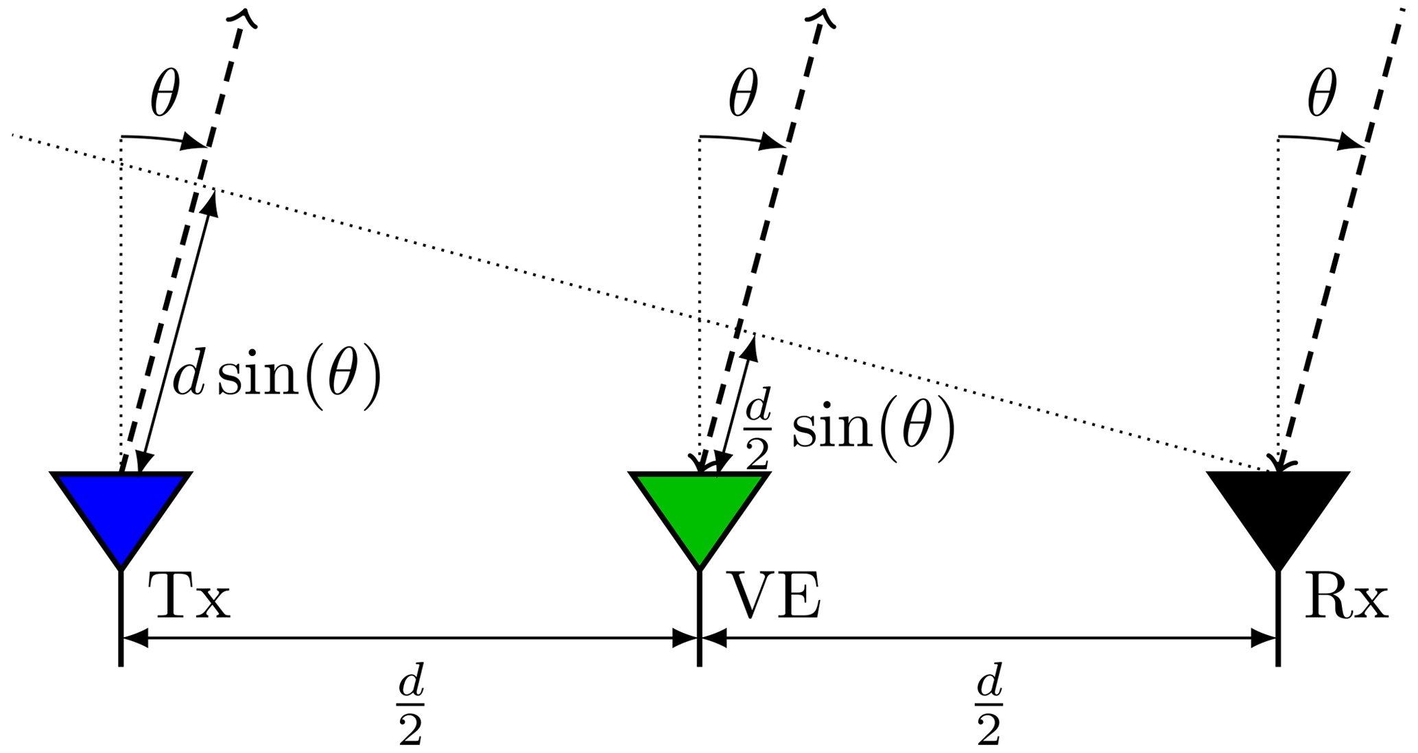
In a bistatic radar scenario, Tx and Rx are distinct antennas at different locations. If the distance R to a target is large compared to the distance d between both antennas, the geometric relationship can be simplified as shown in Fig. 1. The elevation angle θ is the same for both Tx and Rx. The total path Lbi of a plane wave is then
An imagined monostatic antenna midway between Tx and Rx leads to the same total pathlength. This relation also holds for an azimuth angle ϕ unequal to zero. For a large relative target distance R, the Tx-Rx pair can therefore be viewed as a virtual monostatic antenna (Chen and Vaidyanathan, 2009), a so-called virtual element (VE).
2.2 Convolution and scaling
If several Rx and Tx are used together, they form a MIMO system. To allow for the separation from different Tx after reception, the antennas are fed with orthogonal waveforms. Examples of orthogonal waveform strategies are time division multiplex (TDM) (Ender and Klare, 2009) and orthogonal frequency division multiplex (OFDM) (Krieger et al., 2008). Each of the NRx receiver antennas is able to separate the target responses from the NTx transmitter antennas. Therefore, each of the NTx⋅NRx combinations results in a VE, together forming a VA. To analyze the structure of a VA, the method of convolution and scaling can be used. First, the Rx and Tx antenna distributions are expressed as continuous spatial functions FRx and FTx, respectively. These functions possess Dirac spikes at the positions, where an antenna is located. Second, as shown in Ender and Klare (2009), the virtual antenna array is now calculated by convolving scaled versions of the two functions
where (∗) denotes a 2D convolution.
The main focus of this paper is to introduce a simple design method for an equidistant and equally weighted VA along x. Such a VA has the form
with size L and a scaling factor k. The overall length of the VA is k(L−1). The VA forms a grid along x at yVA. Note, that each element in the sum has a weighting of 1, which means exactly one Tx-Rx pair contributes to this VE location. To obtain functions FTx and FRx, a straightforward method is explained in the following sections.
3.1 Establishment of requirements
In order to generate a regular MIMO array in the required form of Eq. (3) with size L, the prime factorization of L is done first. The P prime factors pi∈ℕ with the property
themselves are of course primes and cannot be divided further. It is recommended to choose L, such that the prime factors pi will not get too large. This adds more design flexibility in the method.
3.2 Theoretical outline
From this point onwards, a mixed basis number system will be introduced. Unlike the well-known decimal, binary or hexadecimal number systems, each digit is assigned its own basis. The number system will be represented by a W-element sequence of numbers , where 〈⋅〉 denotes an ordered, finite sequence of numbers and αi the base of the digit at position i, e.g., a three-digit number with basis will have a binary least significant digit. The most significant digit has base 4 and the one in between is ternary. Counting in this number system would yield 000,001, 010,011, 020,…, 320,321. As seen, the amount of displayable numbers in such a number system is finite. A number y in a mixed basis system can be represented as a concatenation of W symbols in the form
where 𝕊S denotes the set of all displayable numbers in a number system S. The conversion 𝚌𝚘𝚗𝚟(y;S) of an integer y from a number system S into a decimal z is calculated as
Next, each prime factor is either assigned a subscript t for Tx or a r for Rx. This can be notated as
where ⊕ denotes a logical exclusive or operation. The sequence 𝒫 is defined as an ordered list of the annotated prime factors in the form
[t|r] denotes, that either the subscript t or r is chosen for each element, but not both. Note, that the choice of a particular assignment as well as the order of the prime factors in 𝒫 will influence the inner structure of the resulting VA and should be chosen in such a way as to design the most feasible MIMO array. A particular number system S with the ordered prime factors from Eq. (8) is now considered. It is in the form
with P=W. For the Tx and Rx antennas, sets of enumerated numbers 𝒯x and ℛx in the number system of Eq. (9) are created respectively. Therefore, the assignment of subscripts t and r from Eq. (8) is used. For 𝒯x all possible numbers in the number system are listed, where the digits at locations with pi,r are zero. For ℛx respectively, all possible numbers are listed of which the digits di are zero, if . Formally, this can be written as
and
The number of elements in 𝒯x is given by
and in ℛx respectively
Each number in 𝒯x is used as a position coordinate for one transmitter antenna in the MIMO design. In the same way, the elements of ℛx are used as coordinates for the receiving antennas. A MIMO system can have at most one distinct VE location for each Tx-Rx pair. Hence, the number of VEs is limited to in the design method introduced here. Therefore, the separation into Tx and Rx antennas is feasible, as it is capable of producing a MIMO array according to Eq. (3).
All physical antennas lie on a line parallel to the x-axis at yTx for Tx and yRx for Rx respectively. Consequently, every element of the VA is located along y at
The same applies to the x-coordinate for each possible Tx-Rx pair. The spatial scaling of will be irrelevant for the following argument and will hence be disregarded. Each element in 𝒯x and ℛx determines the x-coordinate of one antenna according to
where k denotes the scaling factor from Eq. (3). The VA returned from the Tx and Rx positions, which are now fully determined, satisfies the required form from Eq. (3). This can be seen, when the sum of the x-components of Rx and Tx is performed in the domain of number system S. Any element a in 𝒯x with symbols ti added to any element b in ℛx with symbols ri yields a decimal result
This simplification can be done due to the way, 𝒯x and ℛx are defined. For each digit, either the symbol ti or ri is zero. When computing the sum in S, no carry events are happening and through the enumeration, each number in S is reached exactly once through the combination of each one element from 𝒯x and ℛx. Therefore, the set of all Tx-Rx combinations yields 𝕊S. It follows that a VE for a particular position along the x-axis is generated from exactly one Tx-Rx pair.
3.3 Design examples
To illustrate the working principle of this design concept, two different examples are shown that generate a VA with size L=60. More examples and a more small-step explanation of the method can be found in Holder and Eberspächer (2022). The prime factors of L can be ordered and assigned with the subscripts t or r arbitrarily. For the first run,
is chosen. The used number system is . The elements of 𝒯x and ℛx are given in S and as decimals in Table 1.

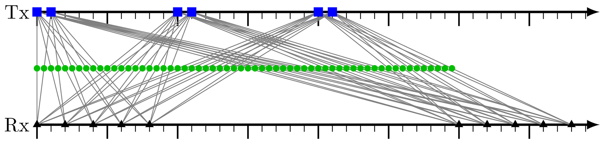
Figure 2Positioning of Tx (blue squares) and Rx (black triangles) antennas along a number line originating from 𝒫1. The resulting virtual elements are shown as green circles.
As a second possible assignment,
is chosen. The used number system here is . The elements of 𝒯x and ℛx for this second example are given in Table 2.
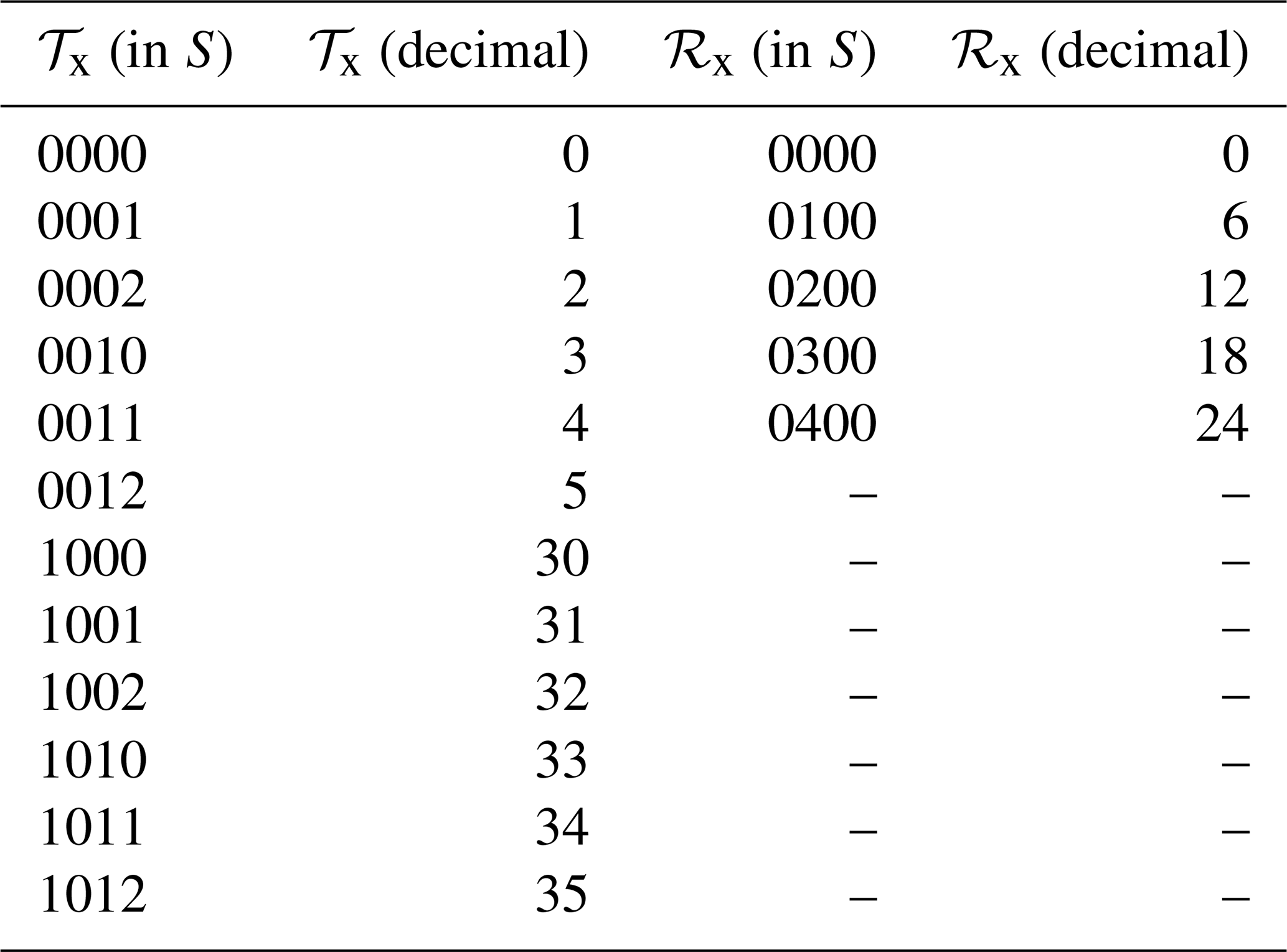
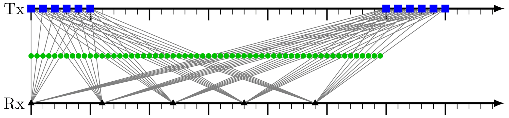
Figure 3Positioning of Tx (blue squares) and Rx (black triangles) antennas along a number line originated from 𝒫2. The resulting virtual elements are shown as green circles.
Figures 2 and 3 show the generated distributions of antennas and their VA for the two exemplary assignments of 𝒫. The first distribution, derived from 𝒫1 in Eq. (17), has six Tx antennas divided into three groups of two. The reason for this structure are the elements 2t and 3t in 𝒫1. The second example has 12 Tx antennas and reveals a completely different structure in Fig. 3. The choice of 𝒫 influences the balance between the number of Tx and Rx and gives the designer some freedom about structuring the antennas into groups. This could be used to meet other design constraints, like a minimum distance between two receivers or minimum total space occupation. A smaller number of Tx antennas facilitates finding a set of orthogonal waveforms. Lockwood et al. (1996) created several MIMO arrays of same size to compare their radiation pattern and beamforming capabilities. However, the uniform MIMO arrays in the paper are just given as examples without any claim about completeness or source. Therefore, a nomenclature is introduced in the following section to properly classify the possible arrays.
3.4 Nomenclature
In the previous sections, a design method for equidistant and equally weighted MIMO arrays was introduced. The designer has two degrees of freedom when deciding for a sequence 𝒫 of subscripted prime factors: The order of the prime factors and their individual assignment to Tx (t) or Rx (r). To classify this design freedom, a nomenclature is proposed. The chain of characters
uniquely identifies a MIMO array. The letter R or T determines, whether this prime factor is assigned to r or t. The subscripts xi give the number system S. Adjacent digits with the same assignment can be accumulated in one digit with a base corresponding to the product of the individual bases, e.g. the subsequence R3R2 will result in the same virtual array as R2R3 or R6. To avoid this ambiguity, each basis should be accumulated such that T and R appear in an alternating fashion. So, the array descriptor T2T2R5R3T3 should be converted to T4R15T3 to increase readability. In favor of generality, arrays with only one Tx or one Rx can be notated as TnR1 or RnT1 respectively. Although strictly speaking they are not MIMO arrays.
3.5 Shifting lemma
Independent of the designed array, shifting all Rx by a spatial vector sRx or all Tx by sTx does not affect the structure of the VA. Tx and Rx positions (encoded as a vector here)
are each shifted by an offset vector. The VA itself is just displaced by the arithmetic mean of sTx and sRx since the resulting position
of the VE is shifted by the same amount for each i<NRx and j<NTx.
The concept of continuously building up antenna groups through digit assignment can also be implemented for the case of a 2D MIMO. In order to create a regular MIMO array in two dimensions, one could either make use of a square grid or a hexagonal grid. A comparison is given by Wagner et al. (2018). Dahl et al. (2017) investigated fractal design approaches on a hexagonal grid, which as well are structured methods to design MIMO arrays of arbitrary size. In this paper, a square grid is used to enable the use of fourier based 3D imaging algorithms (Sheen et al., 2001). For this, the method introduced in the previous section is applied to the vertical and horizontal direction separately. A more practical example is shown using a 80 GHz radar chip.
The goal is to create a 2D MIMO array with the AWR2243 radar transceiver IC from Texas Instruments Incorporated (2020). The chip operates from 76 GHz up to 81 GHz using the FMCW principle. It has three Tx and four Rx channels suitable for MIMO operation. Additionally, multiple chips can be coherently cascaded to operate with an even larger number of antennas. In this example, three chips are used to create an effective size 9×12 MIMO array. To get an array size of Lx=12 and Ly=9, the pattern R2T3R2 is used in horizontal and T3R3 in vertical direction. As the produced MIMO array is intended for direction of arrival (DOA) estimation (Chen et al., 2010), a maximum scaling factor of mm (at center frequency) is allowed theoretically, in order to avoid aliasing. As shown by Zhuge and Yarovoy (2011), this constraint can be relaxed for radar systems with very high fractional bandwidth. The scaling factor k≈2 mm is defined through Eq. (15) since the availible bandwidth is low. The result is shown in Fig. 4. The shifting property from Eq. (21) is used obtain a symmetric design with a common centroid layout. The next step would be to design a patch antenna and to place it at the positions for Rx and Tx. The microstrip routing to the three chips should then be convenient, as the Tx antennas are already clustered in groups of three.
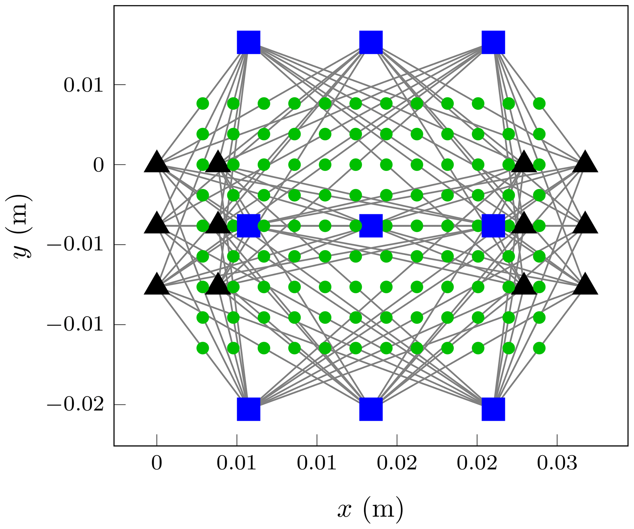
Figure 42D MIMO array design example. Tx positions (blue squares), Rx positions (black triangles) and resulting VA (green circles).

Figure 5Spatially expanded version of the 2D MIMO array design example. Tx positions (blue squares), Rx positions (black triangles) and resulting VA (green circles) are shown.
A drawback of this placement choice is that Rx and Tx antennas are close together in the middle row. Populated with patch antennas, this small physical distance would lead to unwanted crosstalk. Alternatively, Tx and Rx could be separated on the circuit board as shown in Fig. 5 by using the shifting property. This leads to larger overall space requirements, but helps reducing crosstalk. Another solution could be to increase the scaling factor k, if the application can implicitly rule out ambiguities from aliasing by design.
4.1 Analysis of published arrays
Numerous other publications already proposed MIMO arrays, which can be created with this method. Zhuge and Yarovoy (2012) are using a 2D array (R2T3R2 in both vertical and horizontal direction) as a reference for sparse MIMO near-field imaging investigations. Ender and Klare (2009) use an ARTINO type MIMO array in the form T2R44T16, which is installed along the wings of an aeroplane. Another example is a slightly stretched version of a T2R16T8 array (Herschel et al., 2016) for a passenger security system.
This section describes the special case when TRx antennas are used instead of distinct Tx and Rx. First, an alternative view to convolution and scaling, namely polynomial multiplication is introduced.
5.1 Polynomial multiplication
The concept of polynomial multiplication is not only applicable to TRx antennas, but also distinct Tx and Rx, as in Sect. 3. If Tx and Rx antennas are located on a uniform grid with a defined zero-location, the VA can also be calculated via polynomial multiplication. The set of Tx antennas is therefore expressed as a polynomial t(x). A coefficient ci is either 1, if a transmitter antenna is present at this grid point or 0, if not. From the example in Fig. 2, would be returned, while would describe the Rx positions.
The occuring exponents show where Tx antennas are located. The same applies to Rx yielding a second polynomial r(x) with binary coefficients dj. The VA is now computed via polynomial multiplication as
where 𝚍𝚎𝚐(⋅) denotes the degree of a polynomial. The exponent of a term in v(x) indicates the position of the VE while the corresponding coefficient shows, how many Tx-Rx pairs contribute to it. As for the convolution method, the VA has to be spatially scaled by . However, the scaling is not relevant for analyzing the structure of the VA.
5.2 Structured approach for TRx MIMO arrays
If instead of dedicated transmitters and receivers, transceivers are used, the initially proposed methology still works but leads to more redundancy. When each antenna is used as Tx and Rx (TRx), there is no difference between Tx and Rx anymore. This can be understood with the thought, that the sets 𝒯x and ℛx now consist of the set unions
of the initial sets.
The obtained VA from a given regular antenna layout can be represented as the result of a polynomial multiplication. Since the antennas are indistinguishable, holds, where a(x) denotes a polynomial encoding of the TRx positions. Given that the VA is now calculated as
It can be seen from any TRx structure with NTRx≥2 antennas, that redundancy is now implicitly present. The VA originated from two TRx antennas has the form
for an arbitrary positive integer k. The value 2 in the cross-term coefficient shows, that this structure already contains redundancy as two VEs overlay each other at this position.
Let a TRx array with polynomial a(x) have degree n. This means the rightmost TRx element is at position n and the highest nonzero term of a(x) is xn. Assume that the resulting VA does not have any gaps, i.e. vi≥1 for holds for the coefficients vi of v(x). Now consider an extended TRx array, which is composed of a(x) and a shifted copy of a(x). It has the form . The resulting extended VA has the form
Since a(x)2 covers all VE positions from zero up to 2n, the second and third term fully cover the positions ranging from 2n+1 to 4n+1 and from 4n+2 to 6n+2, respectively. By copying and shifting the existing structure, the VA can be extended to three times the original length. This step can be cascaded several times to build up a large VA. The following iterative procedure illustrates this: The first iteration starts with a single TRx antenna represented by a polynomial a0(x)=1 of degree zero. Algorithm 1 shows the procedure to get the TRx MIMO array.
Algorithm 1Iterative method to design a TRx MIMO array.
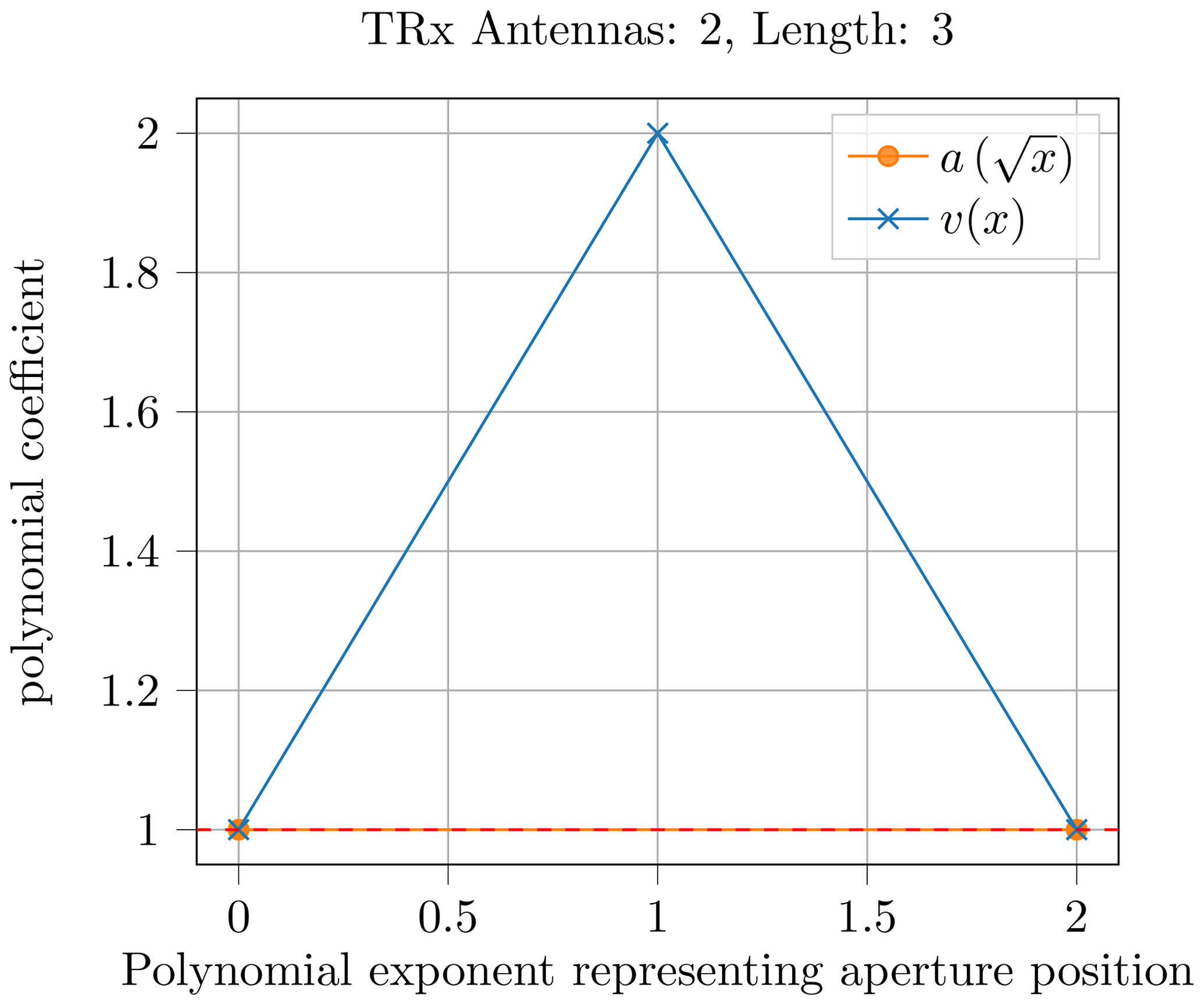
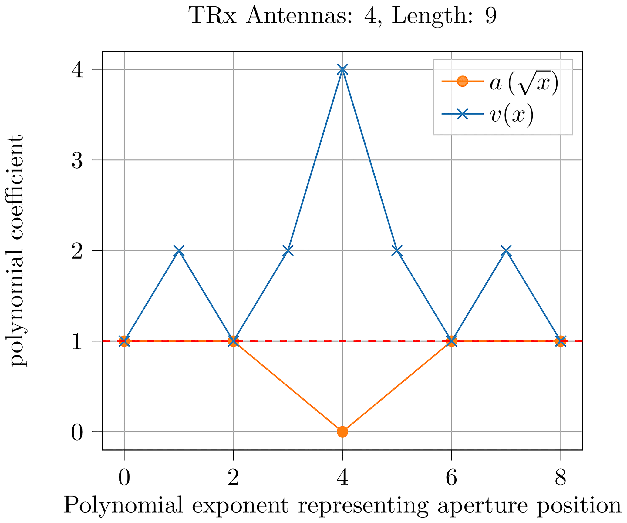

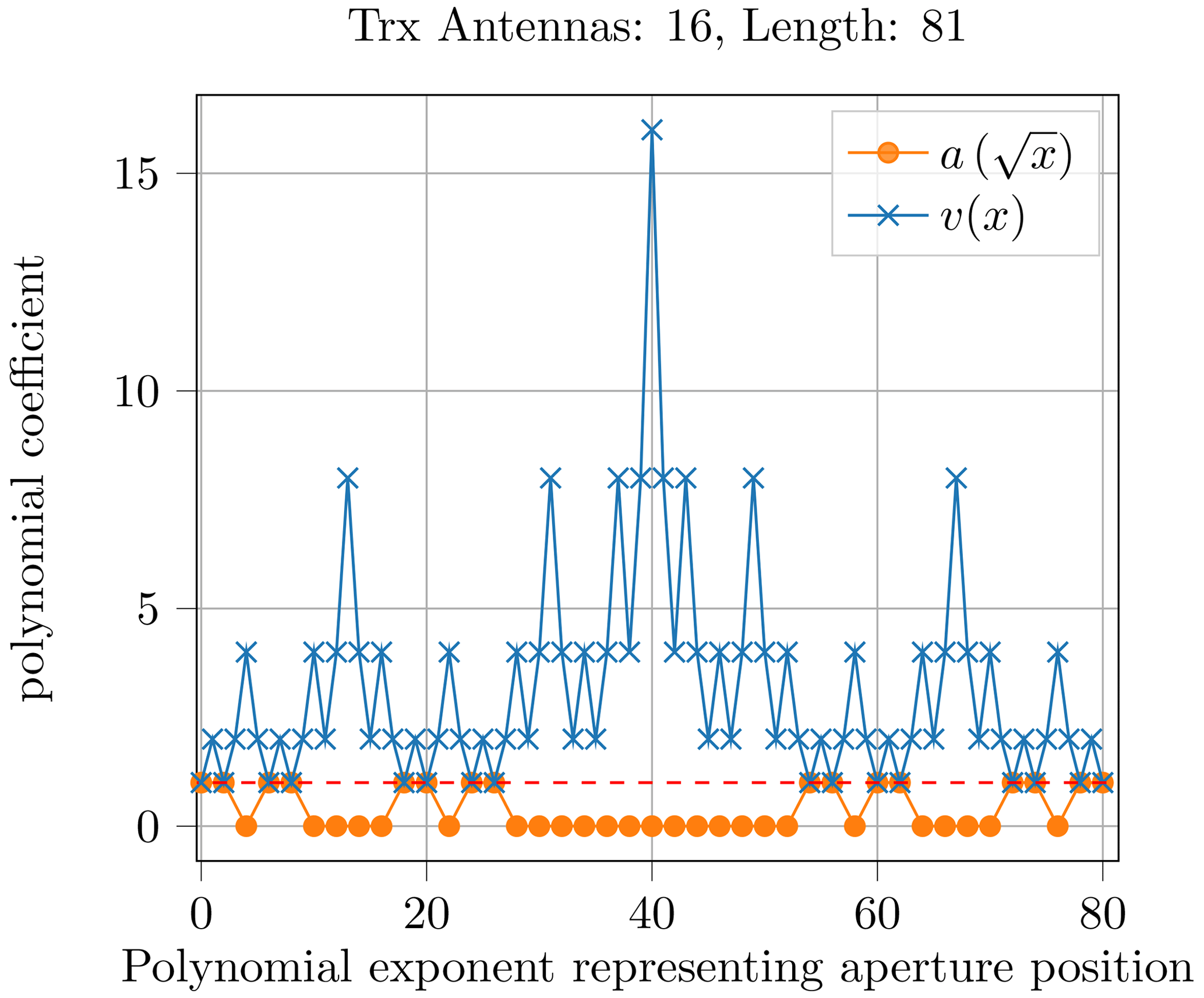
Figures 6 and 7 show the results for Niter=1 and Niter=2 of Algorithm 1. Note that the coefficients of a(x) are shown at stretched positions to visualize the scaling effect, when the VA is generated. Figures 8 and 9 show the coefficients for Niter=3 and Niter=4, respectively. It can be observed that the coefficients get larger over the iterations. While the number of TRx doubles, the MIMO array length is multiplied by three for each iteration.
Compared to the number approach of the previous sections, there are fundamental differences: The redundancy for TRx arrays does increase with the Niter, whereas the number approach was designed to not permit redundancy at all. In exchange, the TRx arrays rely on strictly repeating structures, which lowers the hardware complexity. If the spacing is not feasible inside one iteration, one could always use a smaller shift between the two subarrays to get ae(x). For the iteration, the alternatively produced a(x) from the previous iteration could be used without problems. Additionally, the physical size of the VA coincides with the extent of TRx antennas. For the number system approach, this is never the case.
For a selection of N antennas, the theoretical maximum size L for a regular VA without gaps is for TRx elements. If the antennas are distinct transmitters or receivers, it is . So roughly half of the size is achieved compared to TRx for large N. While the number system approach reaches this limit asymptotically, the outlined approach for TRx elements still has room for improvement.
5.3 Design example
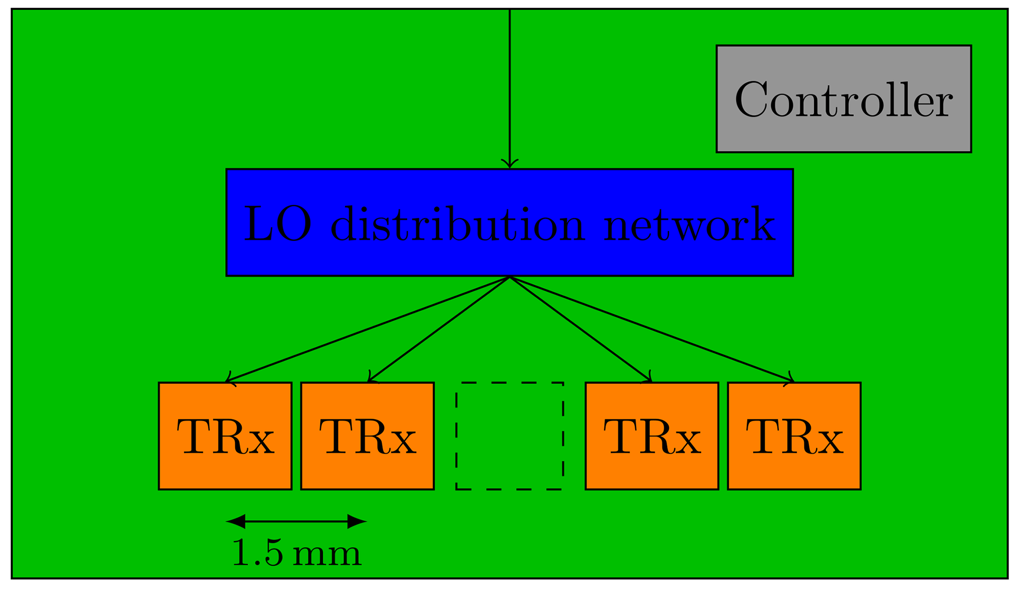
One significant benefit of the approach followed is the resulting modularity of the system. To demonstrate this advantage, a conceived design example is presented in this section. Consider a modular system design, where 16 TRx are used in four modules with four antennas per module. They are operating at a center frequency of 200 GHz. To achieve a sampling density of of the VA at the center frequency, the minimum distance between two TRx is set to 1.5 mm. The transmitter of each TRx can be deactivated to be operated as a receiver only. With only one active transmitter at a time, TDM could be easily realized. Figure 10 shows an outline of such a submodule. It has four TRx antennas arranged in a grid of five with a void element in the middle. Note that this is exactly the obtained structure for Niter=1 in Algorithm 1, shown in Fig. 7.
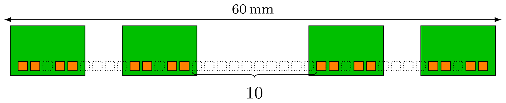
These modules are now placed onto a carrier frame with an arrangement as shown in Fig. 11. First (corresponding to iteration 3 in Algorithm 1) the second module is placed with four units of free space next to the leftmost one. This structure is copied again at the right side. Note, that the free space in the middle is only 10 units wide. However, according to Algorithm 1, it should be 13. It was reduced here to meet an overall maximum length constraint of 60 mm. The resulting VA is therefore reduced in size from 81 to 75. Being able to reduce the shifting distance during one iteration is another benefit of this approach, which increases the flexibility during the design process.
In this paper, two design methods for creating uniform and equidistant MIMO arrays for 1D and 2D applications were introduced. A nomenclature to classify the degrees of freedom in the first method was proposed. Based on a design example for a 2D MIMO array, the versatility of this method was demonstrated. This was underlined by already published designs of other authors, which all could be created with the introduced design method. As a special case, a design method with TRx antennas was introduced and compared. It was shown that redundant virtual elements are implicitly present in this case.
On the other hand, the examples also highlighted limitations of the methods. Design goals and constraints like the physical size of an antenna (and therefore the minimum spacing) or routing constraints are not implicitly considered. Moreover, the special interest of the authors lies in the application of a MIMO structure for near-field imaging. Zhuge and Yarovoy (2011) point out that array factors are position dependant and more complex to determine in a near field scenario, which will be considered in future work. Removing the constraint of equal weighting in the VA, one could either choose to design redundant arrays (L<NVE), sparse arrays (L>NVE) or a combination of both. Both options will be considered in the near future, investigating the effect of an array choice on the realisability and performance of the radar. Especially, the use of a non-convex optimization algorithm lies in the interest of the authors. Another aim of the authors is to find a more elegant and flexible way to design TRx MIMO arrays. A non-trivial two-dimensional extension of the introduced TRx method must be found as well.
No data sets were used in this article.
Both authors conceptualized the ideas of this work. MH carried out the formal analysis and elaborated the methology. He drafted and prepared the manuscript including the visualization of data. ME supervised the work, validated the concepts, reviewed and edited the paper draft.
The contact author has declared that none of the authors has any competing interests.
Publisher’s note: Copernicus Publications remains neutral with regard to jurisdictional claims in published maps and institutional affiliations.
This article is part of the special issue “Kleinheubacher Berichte 2022”. It is a result of the Kleinheubacher Tagung 2022, Miltenberg, Germany, 27–29 September 2022.
The authors would like to thank the innovation department of Balluff GmbH for general support and resource provision for this work.
This paper was edited by Thomas Kleine-Ostmann and reviewed by two anonymous referees.
Chen, Z., Gokeda, G., and Yu, Y: Introduction to Direction-of-Arrival Estimation, Artech house, Norwood, Massachusetts, 46 pp., ISBN 9781596930902, 2010. a
Dahl, C., Rolfes, I., and Vogt, M.: Investigation of fractal MIMO concepts for radar imaging of bulk solids, in: 2017 European Radar Conference (EURAD), 134–137, https://doi.org/10.23919/EURAD.2017.8249165, 2017. a
Ender, J. H. G. and Klare, J.: System architectures and algorithms for radar imaging by MIMO-SAR, in: 2009 IEEE Radar Conference, 1–6, https://doi.org/10.1109/RADAR.2009.4976997, 2009. a, b, c, d
Feger, R., Wagner, C., Schuster, S., Scheiblhofer, S., Jager, H., and Stelzer, A.: A 77-GHz FMCW MIMO Radar Based on an SiGe Single-Chip Transceiver, IEEE T. Microw. Theory, 57, 1020–1035, https://doi.org/10.1109/TMTT.2009.2017254, 2009. a
Gao, J., Qin, Y., Deng, B., Wang, H., and Li, X.: Novel Efficient 3D Short-Range Imaging Algorithms for a Scanning 1D-MIMO Array, IEEE T. Image Process., 27, 3631–3643, https://doi.org/10.1109/TIP.2018.2821925, 2018. a
Herschel, R., Lang, S. A., and Pohl, N.: MIMO imaging for next generation passenger security systems, in: Proceedings of EUSAR 2016: 11th European Conference on Synthetic Aperture Radar, 1–4, ISBN 978-3-8007-4228-8, 2016. a
Holder, M. and Eberspächer, M.: A versatile method to design an equidistant MIMO array, in: 2022 Kleinheubach Conference, 1–4, ISBN 978-3-948571-07-8, 2022. a
Huang, Y., Ma, L., Yu, X., Zhang, H., Li, J., and Xi, X.: MIMO Antenna Array Design Based on Genetic Algorithm, in: 2021 IEEE 4th International Conference on Electronic Information and Communication Technology (ICEICT), 406–409, https://doi.org/10.1109/ICEICT53123.2021.9531259, 2021. a
Krieger, G., Gebert, N., and Moreira, A.: Multidimensional Waveform Encoding: A New Digital Beamforming Technique for Synthetic Aperture Radar Remote Sensing, IEEE T. Geosci. Remote Sens., 46, 31–46, https://doi.org/10.1109/TGRS.2007.905974, 2008. a
Lockwood, G., Li, P.-C., O'Donnell, M., and Foster, F.: Optimizing the radiation pattern of sparse periodic linear arrays, IEEE T. Ultrason. Ferr., 43, 7–14, https://doi.org/10.1109/58.484457, 1996. a
Schmid, C. M., Feger, R., Wagner, C., and Stelzer, A.: Design of a linear non-uniform antenna array for a 77-GHz MIMO FMCW radar, in: 2009 IEEE MTT-S International Microwave Workshop on Wireless Sensing, Local Positioning, and RFID, 1–4, https://doi.org/10.1109/IMWS2.2009.5307896, 2009. a
Sheen, D., McMakin, D., and Hall, T.: Three-dimensional millimeter-wave imaging for concealed weapon detection, IEEE T. Microw. Theory, 49, 1581–1592, https://doi.org/10.1109/22.942570, 2001. a, b
Chen, C. and Vaidyanathan, P. P.: MIMO Radar Spacetime Adaptive Processing and Signal Design, in: MIMO radar signal processing, edited by: Stoica, P. and Li, J., J. Wiley & Sons, Hoboken, New Jersey, 238–242, ISBN 9780470391488, 2009. a
Texas Instruments Incorporated: AWR2243 product page, https://www.ti.com/product/AWR2243 (last access: 26 January 2023), 2020. a
Wagner, J., Barowski, J., Dahl, C., and Rolfes, I.: Comparison between Rectangular and Hexagonal Synthetic Apertures for Radar Imaging, in: 2018 15th European Radar Conference (EuRAD), 150–153, https://doi.org/10.23919/EuRAD.2018.8546654, 2018. a
Yanik, M. E. and Torlak, M.: Near-Field MIMO-SAR Millimeter-Wave Imaging With Sparsely Sampled Aperture Data, IEEE Access, 7, 31801–31819, https://doi.org/10.1109/ACCESS.2019.2902859, 2019. a
Yanik, M. E., Wang, D., and Torlak, M.: Development and Demonstration of MIMO-SAR mmWave Imaging Testbeds, IEEE Access, 8, 126019–126038, https://doi.org/10.1109/ACCESS.2020.3007877, 2020. a
Zhuge, X. and Yarovoy, A. G.: A Sparse Aperture MIMO-SAR-Based UWB Imaging System for Concealed Weapon Detection, IEEE Trans. Geosci. Remote Sens., 49, 509–518, https://doi.org/10.1109/TGRS.2010.2053038, 2011. a, b, c
Zhuge, X. and Yarovoy, A. G.: Study on Two-Dimensional Sparse MIMO UWB Arrays for High Resolution Near-Field Imaging, IEEE T. Antenn. Propag., 60, 4173–4182, https://doi.org/10.1109/TAP.2012.2207031, 2012. a
- Abstract
- Introduction
- Virtual arrays
- Design method for one-dimensional equidistant arrays
- Example design for a two-dimensional array
- The usage of transceiver antennas
- Conclusions
- Data availability
- Author contributions
- Competing interests
- Disclaimer
- Special issue statement
- Acknowledgements
- Review statement
- References