 | 01 Dec 2023
Mathematical optimization and machine learning to support PCB topology identification
Ilda Cahani
Marcus Stiemer
In this paper, we study an identification problem for schematics with different concurring topologies. A framework is proposed, that is both supported by mathematical optimization and machine learning algorithms. Through the use of Python libraries, such as scikit-rf, which allows for the emulation of network analyzer measurements, and a physical microstrip line simulation on PCBs, data for training and testing the framework are provided. In addition to an individual treatment of the concurring topologies and subsequent comparison, a method is introduced to tackle the identification of the optimum topology directly via a standard optimization or machine learning setup: An encoder-decoder sequence is trained with schematics of different topologies, to generate a flattened representation of the rated graph representation of the considered schematics. Still containing the relevant topology information in encoded (i.e., flattened) form, the so obtained latent space representations of schematics can be used for standard optimization of machine learning processes. Using now the encoder to map schematics on latent variables or the decoder to reconstruct schematics from their latent space representation, various machine learning and optimization setups can be applied to treat the given identification task. The proposed framework is presented and validated for a small model problem comprising different circuit topologies.
- Article
(2370 KB) - Full-text XML
- BibTeX
- EndNote


Printed circuit boards (PCB) are laminated sandwich structures of conductive and insulating layers connecting electronic components to one another that are used in almost every electronic product nowadays. The designing of PCBs can, however, be a very challenging task as it often takes a great deal of knowledge and time to position hundreds of components and thousands of tracks into an intricate layout that meets a whole host of physical and electrical requirements (Jones, 2004). As such, proper PCB design is an integral part of value added. There are three important factors to be considered when designing a PCB: power integrity (PI), electromagnetic interference (EI), and signal integrity (SI), e.g., Archambeault and Drewniak (2013), of which will be the focus of this paper.
The availability of powerful simulation tools supporting the different phases of PCB design, i.e., generation of a schematics, placement of components (or modules), routing, and testing with respect to SI, PI, or EI, is essential for modern PCB design, e.g., Jansen et al. (2003), Wang et al. (2009). However, in spite of the accessibility of such methods the extreme size of the configuration space makes PCB design still a hard and time-consuming task. For that reason, various approaches to the application of mathematical optimization and, particularly, machine learning to support electronics design have been recently undertaken, see, e.g., Li et al. (2021), Huang et al. (2021).
Optimization and machine learning are both powerful problem-solving tools as long as the required type, quality, and quantity of data can be provided and sufficient – sometimes extensive – computing resources are available, particularly in case of real world problems. While an optimization method searches for good parameters in the design space by forecasting the shape of its target (or cost) function to be minimized on the configuration space based on its actual state, the aim of machine learning is to deduce abstract knowledge about a process from a large amount of legacy data. Although a parameter identification task can often immediately be modeled as an optimization problem, it usually requires a cost function with some regularity properties to work effectively. In contrast, machine learning does not require any regularity of data, but usually a large quantity of them and has to be employed in a certain framework to be able to serve to an identification purpose. Such a framework could be given by an optimization algorithm in which the machine learning method takes the role of a surrogate model to speed up the parameter identification. Hence, the typical machine learning approaches, clustering, classification, and model learning via regression, are capable of efficiently supporting a parameter identification framework. More sophistication is introduced by approaches as reinforcement learning, see, e.g, Sutton and Barto (2018), where the policy determining an automated agent's action is optimized with respect to its influence on state variables of a system under consideration.
In any case such algorithms need input data that have to describe the parameter space properly. This is easy for electronics components that can be described by several real numbers, which can be sampled to an input vector. A more complex approach is required, when concurring topologies are to be compared, e.g., in the realm of schematics identification. Using straight forward methods to flatten topology descriptions to vectors frequently leads to non connected configuration spaces, which confront machine learning with a hard task and require very particular optimization techniques. In case of structures that can be represented by graphs such as schematics, Graph Neural Networks (GNN, Hamilton, 2020) can help to overcome this issue: Generalizing the idea of Convolutional Neural Networks (CNN), this class of algorithms allows for transforming graph related data in a simpler, so called latent space, thus flattening the complex information contained in a graph structure. The latent space representation itself is learned from the input data so that under good conditions a latent space arises whose variables still represent the important information of the graph. This learning process is usually achieved by feeding the latent space data generated from graph related data by the GNN, which is employed as an encoder in this case, to a decoder that reconstructs graph related data from latent space data. Training of the encoder-decoder sequence is simple, because the graph related input data can directly serve as labels: a perfect encoder-decoder pair leaves the input data unchanged. After training the encoder-decoder sequence, the decoder can be demounted and any machine learning method (clustering, classification, or regression) or optimization method can be applied on the latent space with the encoder mapping schematics representations into the latent space and the decoder reconstructing schematics from information encoded in the latent space. While applying machine learning on a latent space representation is currently intensively studied, not much research exists about the usability of latent space representations for optimization purposes. A delicate question is if and under which conditions the latent space representation will exhibit sufficient regularity for successful application of mathematical optimization.
This work is devoted to evaluating the potential of mathematical optimization and machine learning for automated design problems whose configuration space comprises various topologies. A simple problem is chosen as a first example to demonstrate the feasibility of different approaches: microstrip lines connecting an emitter to several receivers represented by linearized components, have to be arranged in such a way that a sufficiently good connection is guaranteed. As often done in practical applications the quality of the microstrip line connections are validated via S parameters. At first, an optimization algorithms due to Nelder and Mead (Singer and Nelder, 2009) suitable for a directed search in configuration spaces with low regularity is applied to various topological implementations of the network. Their capability of identifying good designs for the various topologies are studied for the different individual topologies first. Subsequently, a machine learning framework based on a GNN-type approach is presented that offers the opportunity of rapidly providing predictions on the relevant parameters of a proposed circuit design. Without the trouble of designing and validating a PCB-network with the particular topology to be assessed (e.g., using scikit-rf) during the optimization framework, the machine learning model will provide a fitness value that can then be used in an optimization method. Finally, the latent space representation achieved by the GNN, is also directly exploited by an optimization approach using the GNN as encoder. Hence, the main achievement of this work is to provide a method that makes design relevant information hidden in a schematics' topology assessable for machine learning and optimization, thus allowing for treating cross-topology identification problems with standard machine learning and optimization frameworks.
Evolving technology has made it increasingly difficult for system developers to produce and maintain complete, unimpaired signals in digital systems (Bogatin, 2004). In order to generate a signal with good SI, several important issues like dispersion, reflections, noise, jitter, attenuation/high frequency loss, etc. need be considered (Brooks, 2003). SI can be measured in the time domain with an oscilloscope or a reflectometer, and in frequency domain with a spectrum analyzer. Of great importance for the validation of linear components such as transmission lines via frequency domain measurements are S parameters: They describe in general the linear behavior of N-port networks, representing ratios between complex amplitudes of incoming and outgoing waves at the considered ports for specific frequencies, either measured in V, A, or even (representing power waves) with equivalent results. More precise, if an, , denotes the complex amplitude of the incoming wave at the port n, and bn the outgoing wave, the S parameters are defined via the following matrix representation:
where the Snn are the reflection coefficients at port n, as can be seen by setting all incoming waves other than an to zero, and Snm is the transmission coefficient from port m to port n. If a sending device associated to port m=1 serves nrec receiving components, such as, e.g., memory chips, the reflection coefficient S11 at the receiver and the transmission coefficients Sn1, , between the source and the nrec ports assigned to the receiving devices provide an informative insight whether the transmitting system (PCB) is apt for high quality signal transfer.
The aim of this paper when dealing with the S parameters is to minimize the reflections as they cause common-mode interference, meaning that too large reflections reduce the power provided at the receivers and superimpose the reflected interference on the signal (Pupalaikis, 2020). For this paper, simulations of S parameters produced in the frequency domain with the Python library scikit-rf (Arsenovic et al., 2022), which is emulating a spectrum analyzer, will provide labeling to our design proposals.
In order to comprehend how traces and components are laid out on the board, a PCB can be visualized as a network embedded in a physical copper-silicon framework where data must flow from one point to another, making it quite significant to analyze and optimize routing topologies to ensure that SI remains consistent throughout. To present the approach sketched above, we study a simple problem class covering several common PCB routing topologies, visualized in Fig. 1, that are based on the traditional topologies also considered in Chiu et al. (2018). These topologies are different simple configurations for laying components and the connection lines between them. Figure 1a displays a star topology, which uses a central pad or via to link multiple points in a circuit to a signal source. Meanwhile, Fig. 1d, displays a fly-by topology, which is a type of daisy chain connection. The daisy chain type of topology links multiple components together in series. A star topology can be useful in order not to impact the signal by the components as they would in a daisy chain (Chiu et al., 2018).
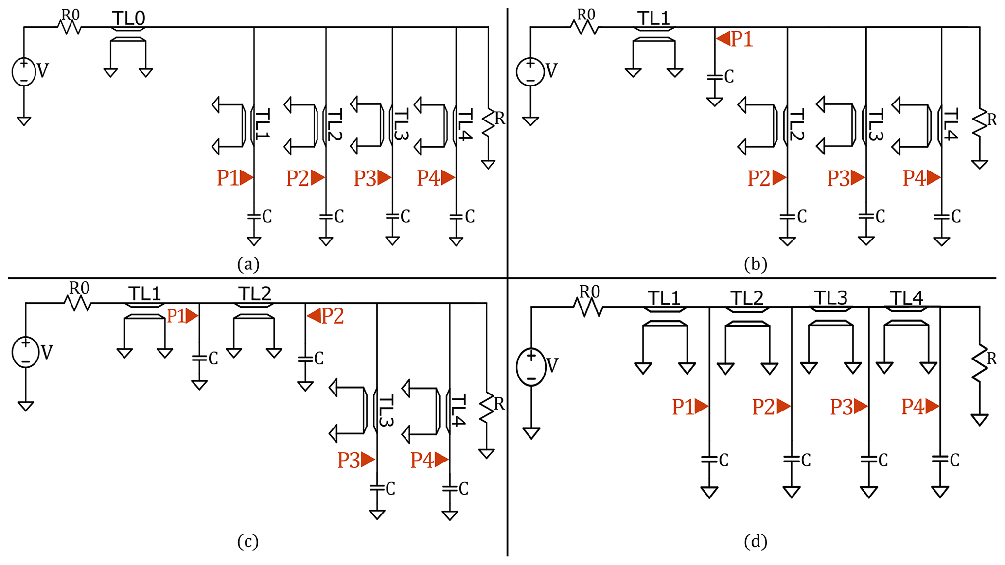
Figure 1Considered topologies: (a) star topology, (b) first mix of star and fly-by topology, (c) second mix of star and fly-by topology, (d) fly-by topology.
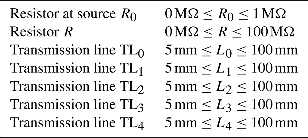
The design of a high quality power distribution network would lead to an analogous consideration. We have also considered mixed versions of these two routing topologies, in order to draw further conclusions on the design choice and open the possibility of more complex topologies being additionally integrated in the optimization process. All four topologies have resistors R0 and R at the extremities with the receivers linked by the transmission lines TL0 to TL4. Highlighted in red in Fig. 1 are the predetermined ports P1 to P4 with S parameters labeled by indices n=2 to n=5. Our aim for this paper is the analysis of these chosen topologies and the minimization of reflections S11 at the emitting port P0 as well as the maximization and equilibration of transmission parameters Sn1, .
Following Chiu et al. (2018), the receiver's load is here simply modeled as a capacitor with a capacitance of C=11 pF. Indeed, a memory module is mainly seen as a capacitive load for the PCB's circuit, where the relevant contribution to its overall capacitance does not come from the small capacitors used to store individual bits of about 25–30 fF (Kim, 1995), but from the packaged/off-chip PCB interconnects between the DRAM memories and processors. For packaged (PoP) interconnects in LPDDR2 memories, Chandrasekar et al. (2013) give a value between 8 and 20 pF, which is in accordance with the value used here. As in this work the general capability of mathematical optimization and machine learning in case of concurring circuit topologies is examined, the choice of the underlying technology and the exact values are of minor importance. In addition, possible non linearities of modules used in practice are not considered here. Accordingly, the S parameter analysis, which is used for circuit validation in this work, does not account for nonlinearities. For large signal circuit designs, non-linear IBIS-files provide a more realistic choice, cf. e.g., Gupta and Chopra (2021).
The microstrip lines used in the four studied PCB topologies are modeled in the frequency range from 100 MHz to 2.6 GHz via the MLine-command of scikit-rf (scikit-rf team, 2022), see also Jahn et al. (2007). They are defined in terms of width WL, thickness TL and height HL between ground plane and conductor comprising a given relative permittivity substrate with permittivity εL (see Table 1) measured at the reference frequency fref=1 GHz.
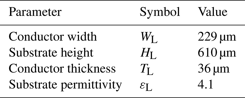
The conductor resistivity is set to and the dielectric loss factor is set to 0. A material roughness of 0.15 µm is assumed. The lengths of the transmission lines is subject to optimization in this work (cf. Table 2). Via the specified material model the frequency depending characteristic impedance Z0 and the transmission delay Td of the transmission lines are determined via an efficient permittivity εeff. The frequency depending S parameters of the microstrip lines can then be determined from these values and employed in the circuit model. More precisely, the quasi-static behavior of the microstrip lines, i.e., at zero frequency, is determined by the Hammerstad-Jensen model with a thickness correction of the microstrip. To account for the frequency dependence (dispersion) of εeff=εeff(f) the Kirschning and Jansen model is applied. Furthermore, for broad band dispersion, also the Djordjevic Svensson correction is activated with parameters flow=1 kHz and fhigh=1 THz.
4.1 Parameter identification via optimization
The optimization algorithm chosen for this specific example is the Nelder Mead simplex search, named after the fact that it starts off with a randomly-generated simplex shape in parameter space, whose corners are given by n+1 parameter tuples, with n being the dimension of the parameter space. Consequently, at every iteration, the algorithm proceeds to reshape and move this simplex towards a more favorable region in the search space applying the two operations reflect and shrink (Singer and Nelder, 2009). As mentioned in the SI section, the target for the chosen example was the minimization of the reflection at the emitting port through
where
is the vector of design parameters to be identified and
is a penalty function quantifying the degree in which design restrictions (constraints), such as minimum length or positivity of physical quantities, are violated. Additionally, m denotes the sample size in frequency space. The minimization of the reflection parameter is demanded in order to minimize unwanted emissions due to common mode disruptions. The design constraints set in this work are listed in Table 2.
Using the Heaviside function ℋ with ℋ(x)=0 for x<0 and ℋ(x)=1, x≥0, they are implemented with the help of the following penalty function (for notational simplicity physical units are suppressed):
With this setting of the penalty convergent solutions to feasible parameters (i.e., such parameters that fulfill the constraints) could be produced. It is a matter of current work if the performance of the algorithm can be enhanced by rendering them all continuous by choosing coefficients before ℋ that assume the value 0 at the switching point and grow moderately as a function of the respective parameter.
The Nelder Mead algorithm searches for local minima. To avoid the algorithm getting stuck in a local minimum and to guarantee a coverage of the whole complex parameter space, the Nelder Mead algorithm is applied several times with different initial parameters that cover the relevant parameter space (see the discussion of the solutions below).
4.2 Optimization results
After 500 steps of the Nelder Mead simplex method optimization, four graphs plotting the S parameters, reflection and transmissions for each port, were produced for each of the considered topologies. The voltage source in Fig. 1 is considered as a sending port with S parameters indexed by m=1. The receiving ports 1–4 (see Fig. 1) are situated in front of the capacity loads 1–4, and will be indexed by integers , as the emitting port will be indexed with m=1. The quantities to be identified through optimization are the values for the resistor R0 and R as well as the lengths for all transmission lines L0 to L4. These are characterized as parameters that minimize the objective function . With a suitable choice of the penalty, the objective should equal the sought reflection parameter in the minimum situation, i.e., the minimum is attained for a feasible parameter.
Observing the evolution of the objective value during Nelder Mead iterations for all four considered topologies in Fig. 2, one notices that low values for the frequency average of are quickly achieved, namely already at the 100th iteration, and the objective value seems to converge for all considered topologies. The high values attained between the 30th and the 80th iteration result from the penalization of constraint violations which fade out in the further iteration process. The results in Fig. 2 allow to conclude that the Nelder Mead iteration finds a local minimum of the objective function, and, hence, of (as constraint violations can be excluded in the optimum situation). To exclude the existence of better solutions in an other part of the configuration space that has not been reached by the iteration, the optimization process has been repeated several times with a couple of different initial values assuring a good coverage of the configuration space. So far, no better results for the frequency average of could be found.

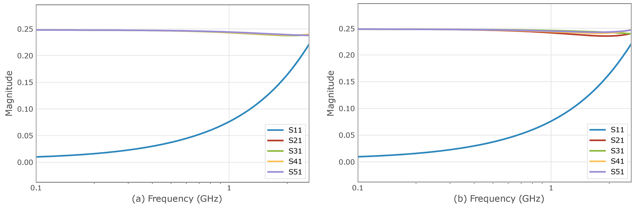
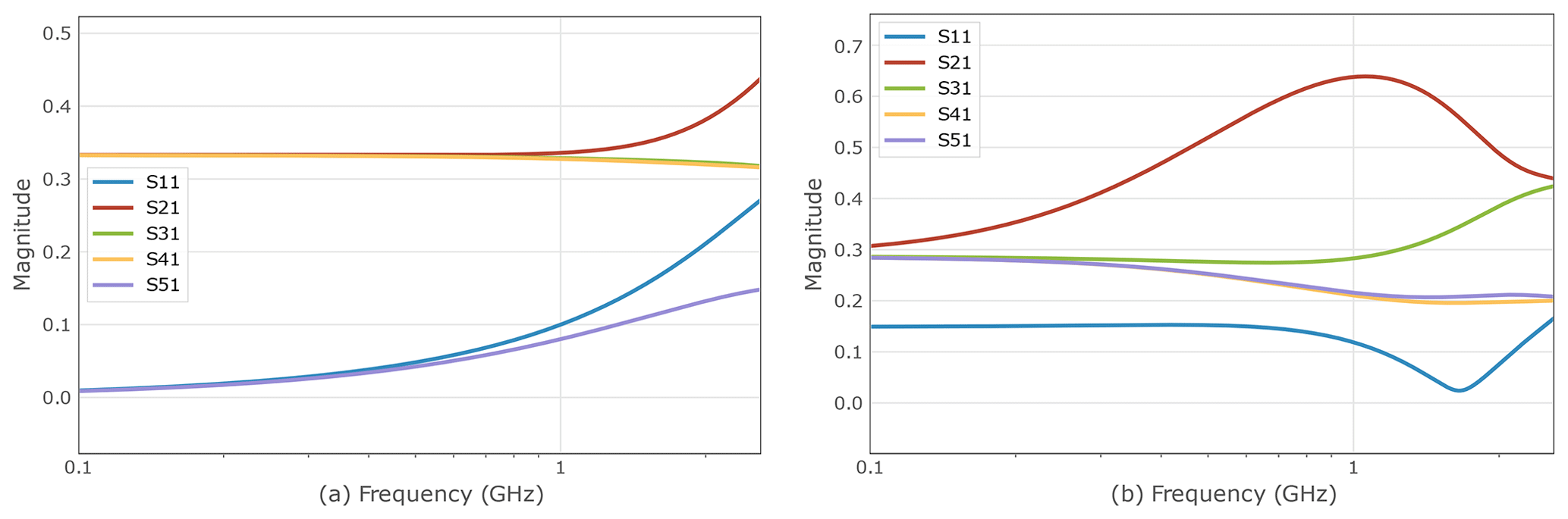

Figure 3 shows the frequency depending S parameters achieved for the first two considered topologies (a) and (b) while Fig. 4 plots the parameters for the last two considered topologies (c) and (d) in Fig. 1. These plotted frequency responses are further supported by Table 3 showing the minimal values achieved by the optimization. One can see from the figures displayed in Fig. 3 and the corresponding parameters representing the optimum configurations displayed in Table 3 that is efficiently reduced close to 0 for lower frequencies. The equality of and implies that no constraint violations occur for the determined optimum values. It is notable that the 4 transmission parameters to stay constantly at the same value 0.25. The equality of the reflection parameters in the optimum situation is self evident for the star topology, but remarkable for the mixed topology (b), as this feature has not explicitly been demanded during the optimization process. However, the magnitude of the reflection coefficient significantly increases with rising frequency from approximately 0.01 at f=100 MHz to more than 0.22 at f=2.6 GHz. The pure star topology exhibits transmission curves slightly closer to each other for the various receiving ports at higher frequencies.
The behavior of the mixed topology (c) plotted in Fig. 4 on the right is similar to those of (a) and (b) with the exception that the average reflection is higher and that the transmission parameter falls under the course of the reflection parameter , while the other three transmission parameters achieve higher values than in the cases (a) and (b) over 0.3. For high frequencies, grows even further.
A completely different picture is seen for the topology (d), plotted in Fig. 4 on the left: In contract to the three first topologies, surpasses here the reflection parameter for the topologies (a), (b), and even (c) for low frequencies, but shows a better high frequency behavior, as it does not increase with higher frequency. The constant behavior over the whole considered frequency range in these cases is a remarkable feature that supports the feasibility of a fly-by topology for high frequency applications. The transmission parameters show quite different behavior, although they all assume uniformly high values over the frequency range. If these variations are to be reduced, an extension of the objective function enforcing more similar transmission coefficients can be implemented.
The method presented in this section and the subsequent results were additionally constructed with a second optimization algorithm due to Powell (1971). For topology (d) where less variation in the course of the transmission parameters has been witnessed in the best configuration found, the results achieved are similar to the Nelder Mead optimization and principally display a lower objective value obtained with longer computing time.
Machine learning (ML) is capable of learning patterns from legacy data by fitting a model, see, e.g., Zhou (2021). It is a well regarded predictive analytics tool, capable of processing massive amounts of legacy data to automatically identify patterns, learn from the data and, thus, make predictions. One significant advantage of ML is how fast it is during the online phase. However, the identification of good designs through ML requires a particular setting. The strategy followed in ML is the minimization of the loss function, which measures the discrepancy of the predicted outcome to measured or simulated values.
5.1 Graph representation
Numerous issues in electronics design can be formalized via graphs. As also represented in Fig. 5, circuit schematics can seamlessly be interpreted as weighted graphs and, thus, benefit from the opportunities offered by machine learning algorithms that are capable of operating with graph structures such as graph neural networks. To represent a schematic as a formal graph, the intersections of conducting connections are represented as nodes and the building elements are specified as weights assigned to the edges lying between the nodes. For simple elements, such as considered in this work, these weights take the from of frequency depending complex numbers. For more complex circuit elements, more complex data, e.g., describing non-linear behavior, are also possible. An electronic network can already be defined by the scikit-rf library, where a particular data structure is provided to represent all electronic components and their connections. However, as evidenced in Fig. 5, the internal data representation employed by scikit-rf is rather complex and, thus, not convenient as a data structure for further processing with the aim to deliver graph information to a machine learning (or optimization) framework. As such, through the use of the Python library Networkx (Hagberg et al., 2008), a complex network can be manipulated into a clearer representation after its creation, so that the resulting structures and connections are ready to be studied by a chosen learning model.
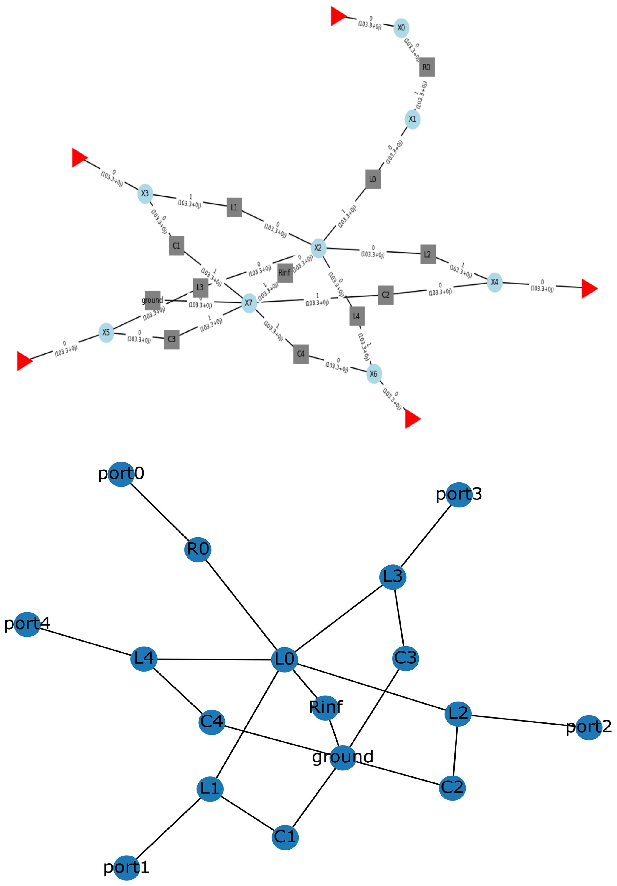
Figure 5Graph representation of the star topology (cf. Fig. 3) through the Python libraries scikit-rf (Arsenovic et al., 2022) and NetworkX (Hagberg et al., 2008).
While GNN libraries allow for direct operation on data in such a graph representation, we opt in this work for transferring the Networkx representation of a schematic further into a two dimensional image format to be able to apply the tremendous wealth of algorithms tailored to treat data in image form directly (see, e.g. Ji et al., 2021). The choice of this approach, which represents in some sense a particular construction method for GNNs, offers the opportunity to customize the applied machine learning algorithms to our particular needs rather than working in a too narrow environment.
To transform the Networkx representation of the given schematics into the realm of image data, it is noted down as an adjacency matrix A={aik}ik, where each node of the graph is related both to a row and a column of the graph. Consequently, each matrix entry represents a possible edge, where rows are considered as starting nodes and columns as terminating rows. An entry aik≠0 indicates that there is an edge starting at node i and terminating at node k. To capture the electronic components linked to the individual edges, the corresponding material values (e.g. complex impedance values etc.) can be stored in the respective positions. This sort of representation of an electronic network assumes the form of an image with the individual entries representing color values of a pixel. As a consequence, the well understood and rich theory of image processing via convolutional neural networks (see, e.g., Ji et al., 2021) applies to these representations of schematics, and the autoencoder methods established for image processing can be transferred to construct latent space representations for schematic, on which machine learning and optimization frameworks can subsequently be implemented.
5.2 Flattened network representation
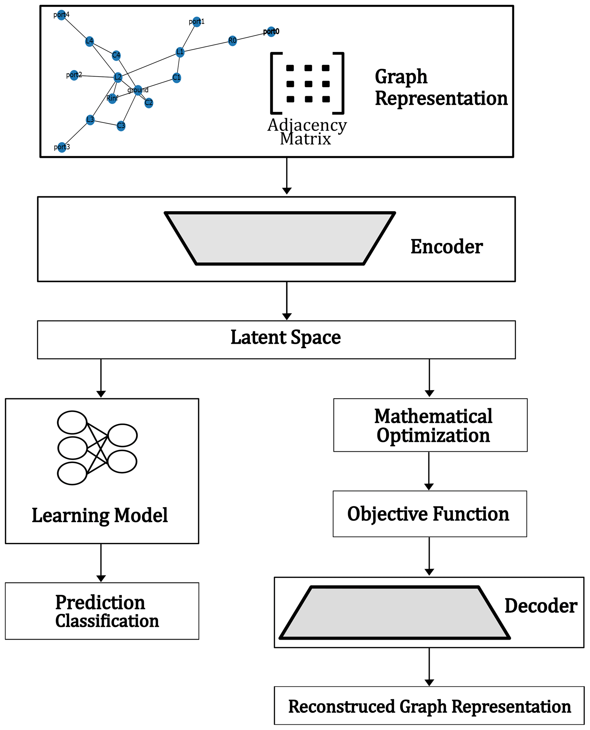
With the preparations from the preceding subsection, complex electronic networks are ready to be modeled or optimized by algorithms directly working on their graph representation. Figure 6 provides a proposal of an electronic design automation (EDA) framework where an encoder-decoder structure (autoencoder) is employed as well as a regression and classification deep neural network: The encoder transforms a weighted adjacency matrix, as defined above, into a vector of defined size d, while the decoder transforms a vector of size d again to an adjacency matrix. The goal of training the encoder and the decoder is to determine a flattened representation of the adjacency matrices, i.e. the latent space (here, the vector space ℝd), that can easily serve as input to machine learning and optimization methods and that contains as much relevant information of the adjacency matrices as possible despite the immense dimensional reduction.
Several ways exist to train such encoder-decoder frameworks. A very practical way is to consider a sequence containing an encoder directly followed by a decoder and to supply a large number of adjacency matrices. The output of the sequence – again being formally an adjacency matrix – is then compared with the input matrix itself, which is also taken as label here, with respect to a suitable metric. In this way, the encoder - decoder sequence is trained to reconstruct identity matrices via a detour through the latent space. After this training, the trained encoder and the trained decoder can be used separately to map adjacency matrices into the latent space and vice-versa. Figure 7 shows on the right hand side the representation of an input graph fed to an autoencoder (from above: scikit-rf representation, adjacency matrix) and on the right hand side the reconstruction from the trained autoencoder. Matrix entries are coded as colors.

Figure 7(b, d) representation of an input graph fed to an autoencoder (from above: schematic, scikit-rf representation, adjacency matrix). (a, c) its counterpart reconstructed by the trained autoencoder.
To construct a GNN, the encoder can be connected upstream to a classifier or a regression model (see Fig. 6). When being trained by adjacency matrices representing schematics the downstream ML method only sees latent space data on which it operates. Such a framework can, on one hand, be applied as a quick computable surrogate model in the context of a mathematical optimization procedure (regression model) or, on the other hand, support the classification between suitable and unsuitable designs. On the other hand, optimization problems can directly be treated on the latent space. The decoder is then required to reconstruct the encoded schematics to obtain objective function values from circuit simulation.
Furthermore, advancing beyond a classification or labeling problem provided by a GNN, a reinforcement learning algorithm would provide continual assessment and corresponding modification of designs through the employment of an agent – an approach well regarded for the considered situations or problems (Sutton and Barto, 2018). Most significantly, this proposed framework would allow for the comparison and validation of new topologies, learning from the graphs that have already been tested.
In this work, the simple structure of the considered PCB topologies allow for restrictions to quite basic ML designs for the employed encoder-decoder frameworks, because parameter sets are small and filtering and regularization steps can be carried out adhoc. Consequently, advanced designs using pooling layers or even stochastic techniques such as in variational autoencoders (e.g., Zhai et al., 2018) are postponed to subsequent studies.
5.3 Machine learning on the latent space
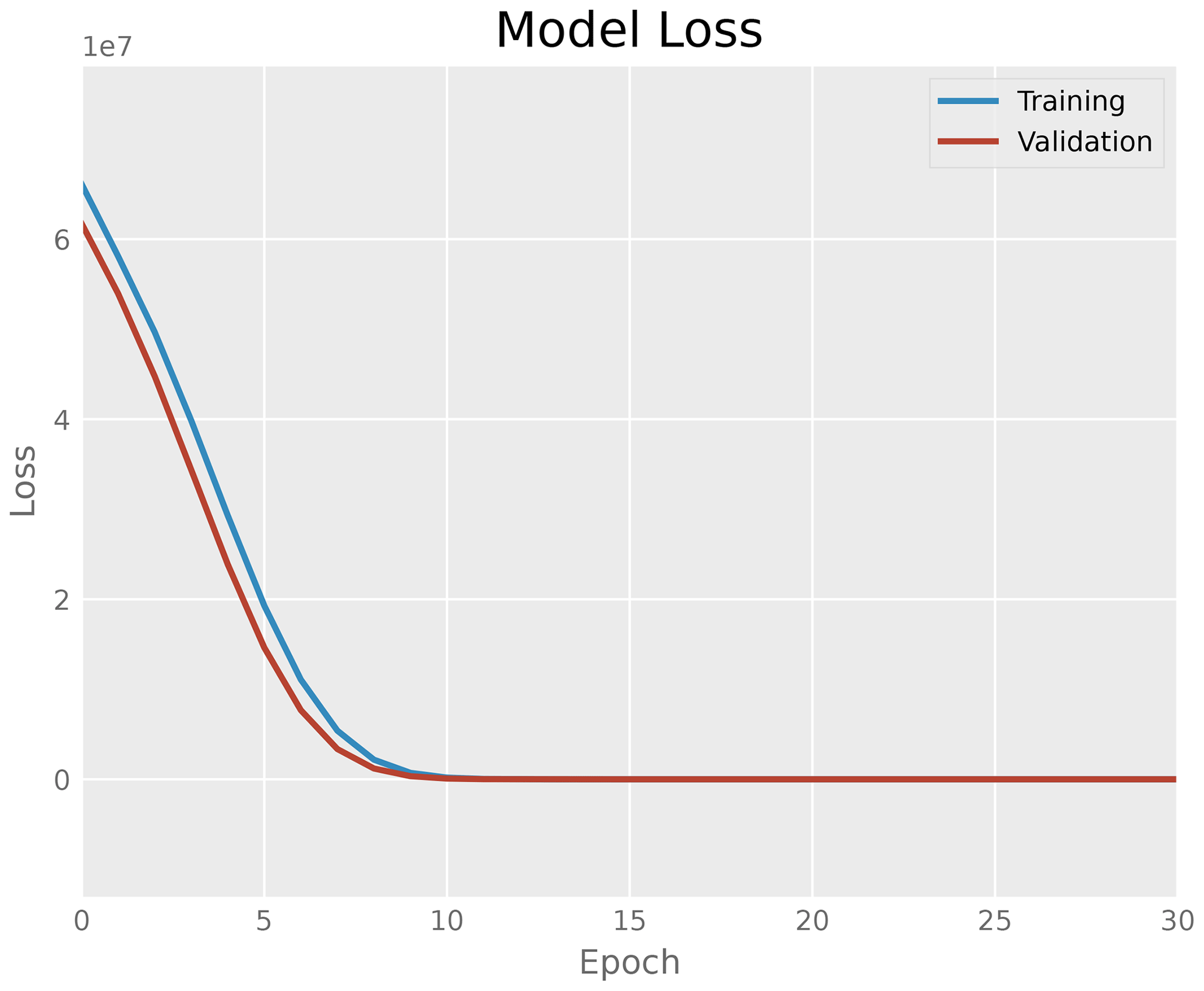
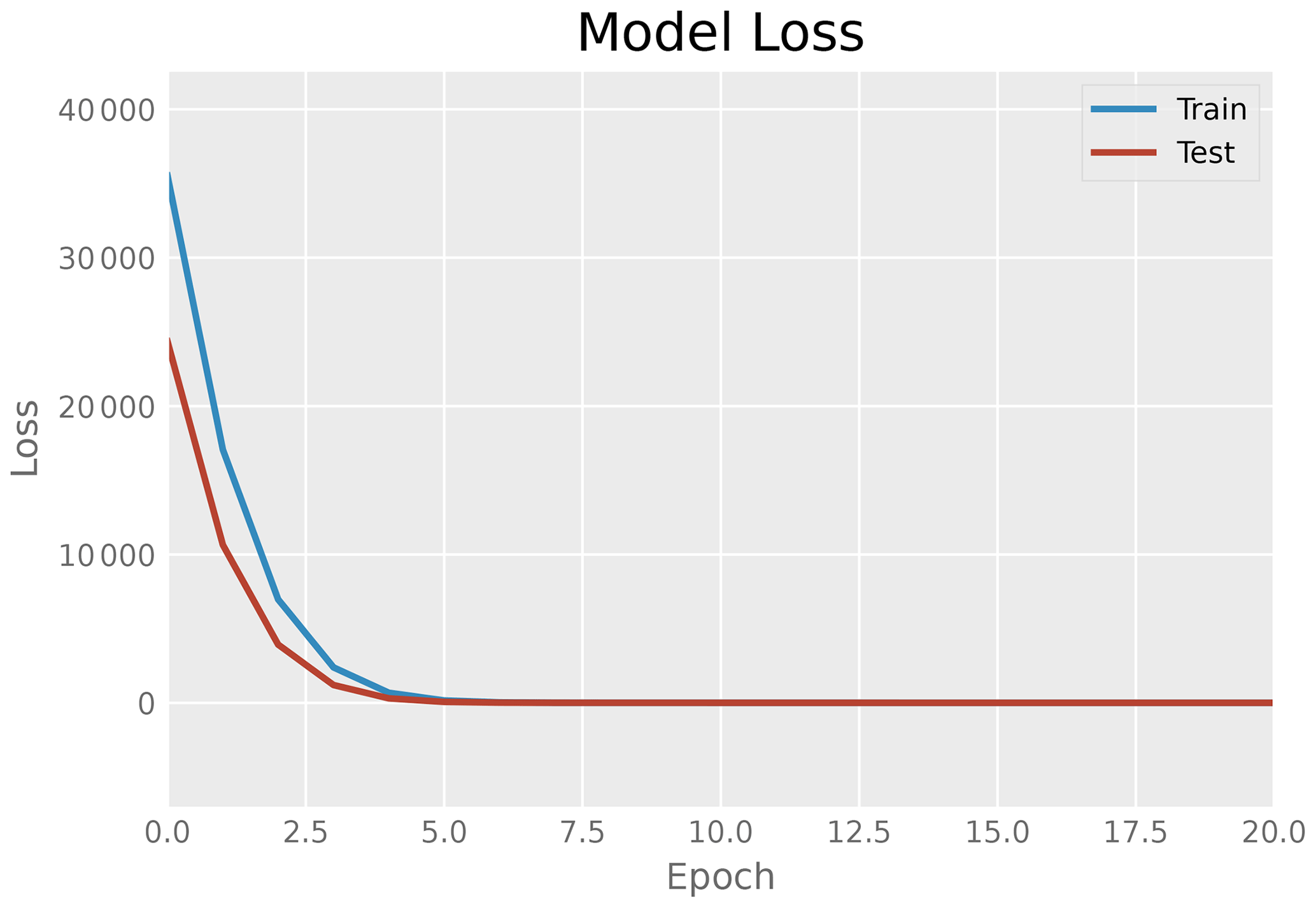
As visualized in Fig. 6, once a graph representation has been constructed for each topology, establishing information of all the aforementioned electronic components and their connections were established, a workflow for the manipulation and lowering of the complexity of the data serving as an input to a learning algorithm is applied. An encoder and a suitable decoder are defined mapping information, such as adjacency matrices of the graphs, to a latent representation of this data and vice-versa. This latent representation is a lower-dimensional compression of the input data onto the latent space, while still maintaining the most important features. A variable d is defined for the dimension of the encoding space. As first simple test version, an encoder with two dense fully connected layers, the first one possessing the dimension of the array the adjacency matrices has been flattened to while the second one possesses the size of the dimension d of the latent space, and a “ReLU” activation function, as well as the corresponding decoder are implemented. In this setting, the latent dimension is set to d=17. The decoder is meanwhile constructed of one dense layer with 289 neurons, a ”ReLU” activation function, and, an additional reshaping layer in order to reconstruct the original data. Figure 8 shows the model loss of the encoder-decoder sequence while learning the latent representation (blue curve) on a sample of 1152 adjacency matrices. The model is compiled with the “Adam” optimizer and mean squared error (MSE) loss function is used for training with the input data. The loss function is reduced dramatically already in the first epochs. In addition, the test-accuracy is plotted in Fig. 8 in red. Showing a similar decay to the training curve, the test curve shows no indication of over-fitting.
Subsequently, the trained encoder is used separately to turn further input data (adjacency matrices) to the latent space representation, and this latent representation is then fed to train a simple deep neural network that is to serve as a regression model. The purpose of this combination is to predict accurately the averaged value of over the considered frequency range, i.e., the objective function considered in the previous chapter for optimization. In contrast to the previously outlined situation, in this case the combination encoder neural network has been trained as one unit. It is believed that a two step approach might be more efficient, which is being currently investigated. The neural network model has two dense layers of 128 and 64 neurons respectively. Figure 9 plots the training loss (blue curve), which indicates the learning of latent data, against the test data (red curve). The labels for the supervised learning process are gained via S parameter computation with scikit-rf for the considered circuits. The weights of the encoder are not chanced during this learning process.
The here presented results are preliminary, in the sense that the research of suitable hyper-parameter values is still subject to research.
5.4 Optimization in latent space
After training of the autoencoder, its decoder part can transform the lower-dimensional representation, in our case that of the latent space, into the original space approximately reconstructing the original input data. This feature can be exploited to have the Nelder Mead (or any other optimization method) run on the latent space. As part of the objective function, the decoder will be evoked whenever an objective value for a data point in the latent space is required. Inside the objective function, some regularization has to be applied to the decoded adjacency matrices, which is done by a simple projection step in the simple examples considered here. Alternatively, a very efficient, yet slightly less accurate scheme can be obtained by using annotations to the original data as labels for the corresponding latent space data and identifying a machine learning surrogate model for the target function on the latent space. For a sufficient amount of more complex data, the autoencoder can be augmented to a more flexible device, e.g., by incorporation of a pooling layer. While the framework has been built up so far, the presentation and analysis of first results represents work in progress. This comprises the discussion of delicate questions concerning the regularity of the objective function as a function of the latent space and its implications for the efficiency of the optimization.
A framework to assist to the modeling, classification, and identification of PCB designs involving different topological approaches is proposed. As a first application of the proposed method, reduction of reflections on simple electronic networks is studied. The underlying idea of the approach is to break down the relevant information hidden in the network structure to a flattened latent space via an encoder-decoder structure. After this variant of graph neural networks has been trained by sufficiently many PCB schematics representations, the encoder and decoder can be employed separately to transfer PCB related data into the latent space, where they can be processed via standard machine learning and optimization frameworks, and, from there, back into a network representation.
In this work, we analyzed the building blocks of the framework sketched above separately with the help of a small problem involving various circuit topologies, i.e., star-topologies, fly-by-topologies, and hybrid variants of them. These building blocks comprise an optimization setup that has been applied in a first step to each considered topology layout. In doing so, we could show that the Nelder Mead simplex search is an example of a feasible optimization method that can be applied on a flattened data structure. It came out that the considered simple model problem comprises sufficient features to be studied in a cross-topology approach: While for the star-like topologies a superior low-frequency behavior, i.e., much lower reflection at the input port, could be achieved via optimization, the fly-by type topologies offered a more stable high frequency behavior with the optimum reflection parameter being nearly independent of the frequency. Hence, it came out that the complexity of the considered topologies is manageable and the Nelder Mead optimization is efficient for the considered PCB topologies.
A second achievement demonstrated in this work is an autoencoder framework that maps after training weighted adjacency matrices of circuits of various topology into a latent space in such a way that the relevant topology information is maintained. This framework shall be employed in two ways: The encoder will be used as upstream component for a simple classification or regression algorithm. Here a first example could be presented. The established regression model allows for determining S parameter information for circuits of various topologies without the need of explicitly constructing the circuit first. Used as a surrogate model in an optimization framework, such a regression model yields a relevant gain in efficiency. The other intended application of the proposed autoencoder is as a downstream component to an optimization algorithm operating on the latent space. Here, it serves as a component in the objective function of the optimizer.
With this paper and the optimization and machine learning methods studied within, we provide a reference for future applications in which different topologies can directly be compared. The focus will be on integrated and automatized schemes to treat various complex approaches in one framework. The proposed application of graph neural network will be followed in further studies, where the benefits of encoder-decoder structures using convolutional neural networks will be further analyzed. Particularly more advanced techniques such as variational autoencoders will be considered. Further points of subsequent studies are the setups of parameter identification frameworks on the latent space, such as the use of machine learning models as surrogate models in an optimization method or a reinforcement learning process.
Due to ongoing refinement and optimization, the code is not yet published.
All relevant models and results of the research are contained in the manuscript, the work can be reproduced with the presented descriptions, formulas, and Python libraries.
IC programmed the computer code, did the data analysis, and provided the graphical representation of the results. Both authors planned the study together, discussed the results, and contributed to the text.
The contact author has declared that neither of the authors has any competing interests.
The responsibility for this publication is held by the authors only.
Publisher's note: Copernicus Publications remains neutral with regard to jurisdictional claims made in the text, published maps, institutional affiliations, or any other geographical representation in this paper. While Copernicus Publications makes every effort to include appropriate place names, the final responsibility lies with the authors.
This article is part of the special issue “Kleinheubacher Berichte 2022”. It is a result of the Kleinheubacher Tagung 2022, Miltenberg, Germany, 27–29 September 2022.
This work is funded as part of the research project progressivKI https://www.edacentrum.de/projekte/progressivKI (last access: 25 September 2023).
This research has been supported by the Bundesministerium für Wirtschaft und Klimaschutz (grant no. 19A21006R).
This paper was edited by Jens Anders and reviewed by two anonymous referees.
Archambeault, B. R. and Drewniak, J.: PCB Design for Real-World EMI Control, vol. 696, Springer Science & Business Media, https://doi.org/10.1007/978-1-4757-3640-3, 2013. a
Arsenovic, A., Hillairet, J., Anderson, J., Forstén, H., Rieß, V., Eller, M., Sauber, N., Weikle, R., Barnhart, W., and Forstmayr, F.: scikit-rf: An Open Source Python Package for Microwave Network Creation, Analysis, and Calibration [Speaker’s Corner], IEEE Microwave Magazine, 23, 98–105, https://doi.org/10.1109/MMM.2021.3117139, 2022. a, b
Bogatin, E.: Signal and Power Integrity: Simplified, Prentice Hall Professional, 2nd edn., https://doi.org/10.1007/978-1-4757-3640-3, 2004. a
Brooks, D.: Signal Integrity Issues and Printed Circuit Board Design, Prentice Hall modern semiconductor design series, Prentice Hall Professional, ISBN 2003046969, 2003. a
Chandrasekar, K., Weis, C., Akesson, B., Wehn, N., and Goossens, K.: System and circuit level power modeling of energy-efficient 3D-stacked wide I/O DRAMs, in: 2013 Design, Automation & Test in Europe Conference & Exhibition, 18–22 March 2013, Grenoble, France, pp. 236–241, IEEE, https://doi.org/10.7873/DATE.2013.061, 2013. a
Chiu, C.-C., Yang, K.-Y., Lin, Y.-H., Wang, W.-S., Wu, T.-Y., and Wu, R.-B.: A novel dual-sided fly-by topology for 1–8 DDR with optimized signal integrity by EBG design, IEEE T. Compon. Pack. T., 8, 1823–1829, 2018. a, b, c
Gupta, A. and Chopra, A.: Impact of DBI Feature on Peak Distortion Analysis of LPDDR5 at 6400Mbps, in: 2021 IEEE 71st Electronic Components and Technology Conference (ECTC), 1–4 July 2021, San Diego, CA, USA, pp. 1838–1843, IEEE, 2021. a
Hagberg, A., Swart, P., and S Chult, D.: Exploring network structure, dynamics, and function using NetworkX, Tech. rep., Los Alamos National Lab. (LANL), Los Alamos, NM (United States), 2008. a, b
Hamilton, W. L.: Graph representation learning, Synthesis Lectures on Artifical Intelligence and Machine Learning, 14, 1–159, 2020. a
Huang, G., Hu, J., He, Y., Liu, J., Ma, M., Shen, Z., Wu, J., Xu, Y., Zhang, H., Zhong, K., Ning, X., Ma, Y., Yang, H., Yu, B., Yang, H., and Wang, Y.: Machine learning for electronic design automation: A survey, ACM Transactions on Design Automation of Electronic Systems (TODAES), 26, 1–46, 2021. a
Jahn, S., Margraf, M., Habchi, V., and Jacob, R.: Qucs technical papers, Qucs-Project, https://qucs.sourceforge.net/docs/technical/technical.pdf (last access: 5 February 2023), 2007. a
Jansen, D., Schütz, A., Voland, G., Stockmayer, F., Kreutzer, H., Rülling, W., Nielinger, H., Prochaska, E., Rieger, M., Schwarz, P., Paul, U., Clauss, H., Albert, G., Toepfer, H., Schuster, G., Foitzik, A., and Kohlhammer, B.: The Electronic Design Automation Handbook, Springer, https://doi.org/10.1007/978-0-25 387-73543-6, 2003. a
Ji, Y., Zhang, H., Zhang, Z., and Liu, M.: CNN-based encoder-decoder networks for salient object detection: A comprehensive review and recent advances, Information Sciences, 546, 835–857, 2021. a, b
Jones, D. L.: PCB design tutorial, 29 June, 3, 25, http://alternatezone.com/electronics/files/PCBDesignTutorialRevA.pdf (last access: 7 February 2023), 2004. a
Kim, C.: Basic DRAM Operation, https://people.eecs.berkeley.edu/~pattrsn/294/LEC9/lec.html (last access: 7 February 2023), 1995. a
Li, Y., Lei, G., Bramerdorfer, G., Peng, S., Sun, X., and Zhu, J.: Machine learning for design optimization of electromagnetic devices: Recent developments and future directions, Appl. Sci., 11, 1627, https://doi.org/10.3390/app11041627, 2021. a
Powell, M. J.: Recent advances in unconstrained optimization, Mathematical programming, 1, 26–57, 1971. a
Pupalaikis, P. J.: S-parameters for Signal Integrity, Cambridge University Press, https://doi.org/10.1017/9781108784863, 2020. a
scikit-rf team: skrf.media.mline.MLine, Tech. rep., sciki-rf, https://scikit-rf.readthedocs.io/en/latest/api/media/generated/skrf.media.mline.MLine.html (last access: 23 November 2023), 2022. a
Singer, S. and Nelder, J.: Nelder-mead algorithm, Scholarpedia, 4, 2928, https://doi.org/10.4249/scholarpedia.2928, 2009. a, b
Sutton, R. S. and Barto, A. G.: Reinforcement learning: An introduction, MIT press, https://doi.org/10.1109/TNN.1998.712192, 2018. a, b
Wang, L.-T., Chang, Y.-W., and Cheng, K.-T. T.: Electronic design automation: synthesis, verification, and test, Morgan Kaufmann, https://doi.org/10.1016/S1875-9661(08)X0006-4, 2009. a
Zhai, J., Zhang, S., Chen, J., and He, Q.: Autoencoder and its various variants, in: 2018 IEEE international conference on systems, man, and cybernetics (SMC), IEEE, 415–419, 2018. a
Zhou, Z.-H.: Machine learning, Springer Nature, https://doi.org/10.1007/978-981-15-1967-3, 2021. a
- Abstract
- Introduction
- SI issues and measurements
- PCB design with various topologies
- Mathematical optimization
- Machine learning
- Conclusions
- Code availability
- Data availability
- Author contributions
- Competing interests
- Disclaimer
- Special issue statement
- Acknowledgements
- Financial support
- Review statement
- References