 | 01 Dec 2023
MmWave scattering properties of roads on rough asphalt and concrete surfaces
Vera Kurz
Manuel Fuenfer
Florian Pfeiffer
Erwin Biebl
In this work, a synthetic aperture radar setup is used for analyzing the mmWave scattering of road surfaces in the automotive 77 GHz band in the laboratory. With this setup, samples of concrete roads in two different surface conditions are investigated, determining the variances in reflectivity depending on material composition and surface structure. Afterward, the distribution of these variations is fitted using probability density functions, namely normal and rayleigh distribution fits. Consequently, the diffuse scattering behavior of concrete roads can be described mathematically. Additionally, previously presented porous asphalt roads are compared and fitted analogously to get a summary of the scattering for all common road surfaces in Germany. Furthermore, a validation of the measurement and the processing by analyzing particularly generated reference samples is performed.
- Article
(5592 KB) - Full-text XML
- BibTeX
- EndNote


The automotive industry is one of the most important branches of industry in Germany. Current developments are moving in the direction of increasingly automated driving. For a safe development of highly-automated driving functions, the ability of sensor and scenario simulation is essential, as it reduces the effort in comparison to real-world testing (Winner, 2018). Such simulations can cover single sensors or can be a fusion of various sensors. Widely used sensors are e.g. cameras, infrared cameras, lidar, and radar sensors. Since there are few data sets of radar sensors as well as few data determining the scattering behavior of particular materials for radar measurements, the setup of such simulations can be difficult. Basic approaches like in Hirsenkorn et al. (2017) in Wald and Weinmann (2019) often use only geometrical optics and ray tracing, ignoring varying material properties in the scenario. Implementing material properties in simulations can improve the accuracy of the results or leave resources at critical points by reducing the computational effort of strongly attenuated reflections. This work concentrates on roads, as they are a relevant environmental element in automotive scenarios. More than 20 years ago, Li and Sarabandi (1999) already analyzed road backscattering using a 94 GHz polarimetric radar system. Anyways, they did not distinguish between various asphalt types but summarized the surfaces in three categories. This results in an examination of rough and smooth asphalt as well as smooth concrete without further differentiating. Furthermore, these investigations are not performed for the automotive 77 GHz band. Schneider et al. (2000) also worked on radar road scattering, mainly considering weather conditions like snow or rain covering the road. The road itself is generalized, assuming one special type of asphalt that is characterized accurately. Thus, information about differences caused by varying road surfaces and material composition are not considered yet but will be analyzed in the following section.
As mentioned before, e.g. a polarimetric radar system can be used for obtaining scattering data. Another common method to gain information about surfaces, especially if they should be very accurate, is using a synthetic aperture radar (SAR). However, past work using SAR on road characterization concentrate on road condition, like Babu and Baumgartner (2020), who monitor mainly road damage. The recorded inhomogeneities are of higher order than for this work. Finally, there are various investigations on detecting roads in satellite SAR images. Anyways, these detections do not differentiate through material properties but use image processing for that purpose. E.g. Henry et al. (2018) use segmentation for detections.
SAR data is primarily processed to images. But when statistical effects are an issue like in Mahapatra et al. (2015), using probability distributions for comparison is convenient. Therefore, in the following section, a SAR measurement setup is shown, validated, and used to complete the measurement series on common road surfaces built in on German highways to get a full set of distribution of all these surfaces. This study is an extension of the work of Kurz et al. (2021) and Kurz and Biebl (2022). Kurz et al. (2021) analyzes the reflection of the different road surfaces for cases when specular reflection can be assumed. However, it becomes clear in this work that road surfaces up to very high angles of incidence cannot be assumed to be smooth, and thus diffuse reflection can occur. After radar is also used for near range applications, this also occurs in practice. With this work and the two previous ones, the reflection behavior should be covered for diffuse as well as specular reflection. The resulting description can be integrated into a statistical model for simulation. An example where this could be helpful is small obstacle detection, as this is mainly done in short distances. In order to record the diffuse scattering as well as possible, an incidence angle of 0∘ is selected. With using a SAR system, the scattering can be averaged over small deviating angles.
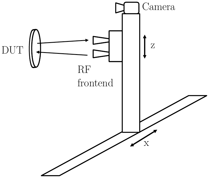
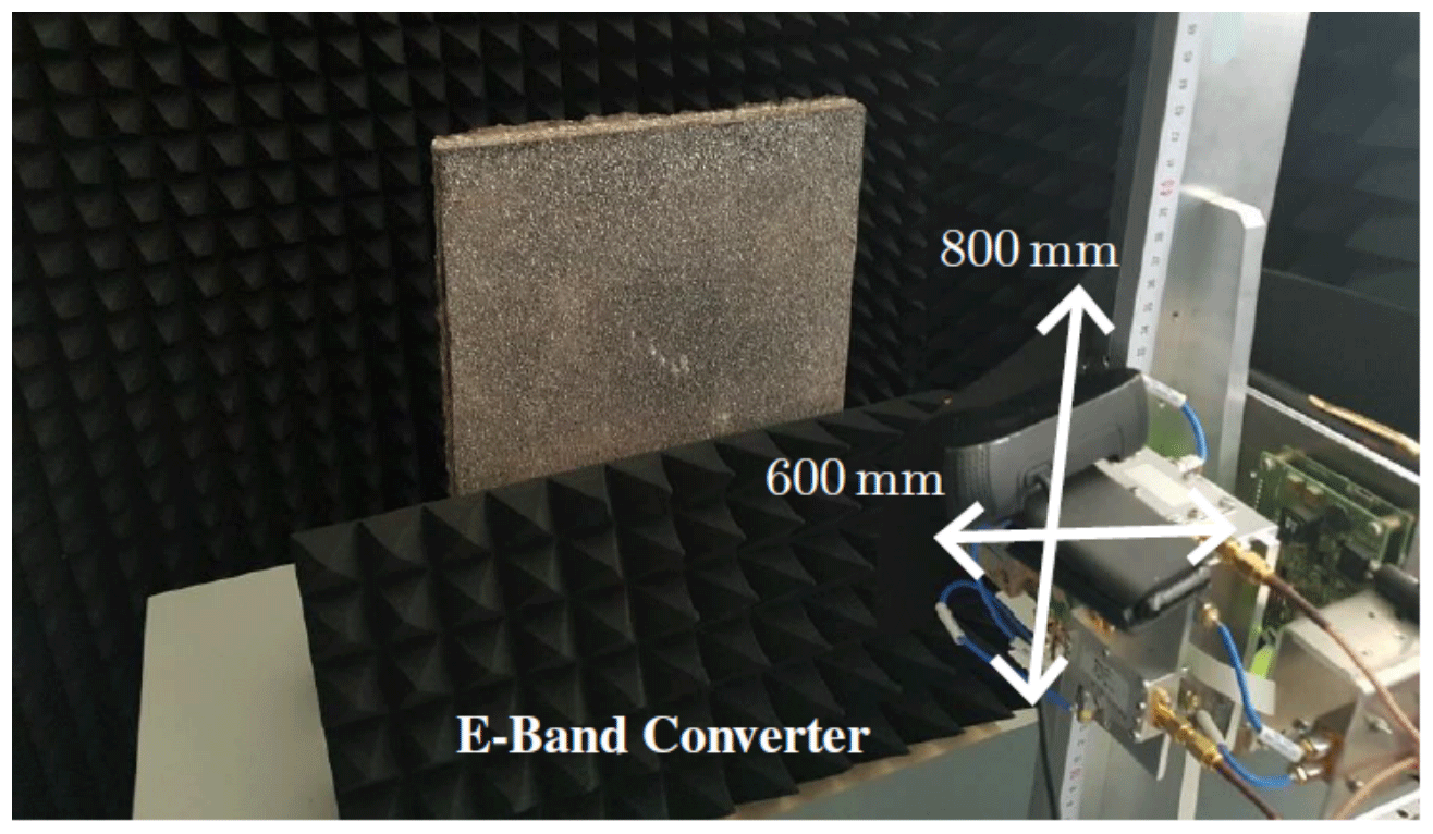
For this investigation, a SAR is used, with which, in the end, a 3D radar reflection image can be calculated by means of a back projection algorithm. The actually measured sample is fixed directly opposite to two antennas, one transmitting and one receiving, which put up the RF frontend. Its mounting stage moves in x and z direction from one measurement point to the other, performing a quasi-static measurement. Therefore, the wave travels from the transmitting antenna to the sample, where it is reflected back to the receiving antenna. This setup is illustrated in Fig. 1. Thus, the transmission (S21) between both antennas is recorded in amplitude and phase. The measurement is realized in a frequency range of 75.7–77.7 GHz in horizontal polarization. The setup accomplishes a synthetic aperture of 800 mm × 600 mm with a step size of 1.6 mm. As reflections from the environment can influence the measurement, the fixture of the sample under test as well as the surrounding, is covered with pyramidal absorbers. The distance between probe and frontend is determined manually, and a camera on top of the frontend assures detailed documentation. The final laboratory collocation is depicted in Fig. 2. The samples are scanned both from the rear and the front side. As the back side is plain, its analysis offers information about material differences in scattering, while the front side shows the influence of the surface structure. In all measurements, a metal washer is placed in the analyzed area. Assuming that it is perfectly reflecting, it is used as a calibration value for a reflectivity of 0 dB.
During this work, two kinds of sample groups are analyzed. One is for an additional validation of the setup and samples of concrete, how it can be found on German highways and streets.
3.1 Reference samples
In order to validate the measurement setup, two reference samples are structured, for which the two appearing distribution functions can be presumed. The first one consists of a smooth aluminum plate, which is surrounded by a plastic frame serving as casting mold. The mold is filled with epoxy resin, and in the liquid resin bearing balls are distributed randomly. The epoxy resin has an expanse of 10 cm × 10 cm × 0.9 cm. For determining the attenuation of a wave in this material, it was analyzed in a focus-beam transmission measurement presented by Pfeiffer et al. (2008). The resulting curve over the frequency is shown in Fig. 3. Matching the measured attenuation of the epoxy resin to its thickness of the reference sample, an attenuation of −8.1 dB is expected, assuming full reflection on the aluminum plate. As the scattering of a rough surface is analyzed, the bearing balls should be smaller than the resolution of the setup. Therefore, a bearing ball diameter of half the wavelength, thus 2 mm, is selected. For the preparation of the reference sample, 1500 bearing balls are thrown in the air in order to create a random distribution. The ones falling away from the samples are collected and thrown again, but the ones near to the samples are not removed before complete hardening to prevent irregularities in the probe surface. This results in a total amount of 1442 bearing balls distributed over the sample. The final distribution can be seen in Fig. 4. The normal distribution is used for a great diversity of phenomena, for example, for modeling random distributions (Forbes et al., 2011). As the scattering objects are distributed randomly, the analysis should result in a normal distribution.
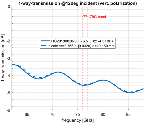
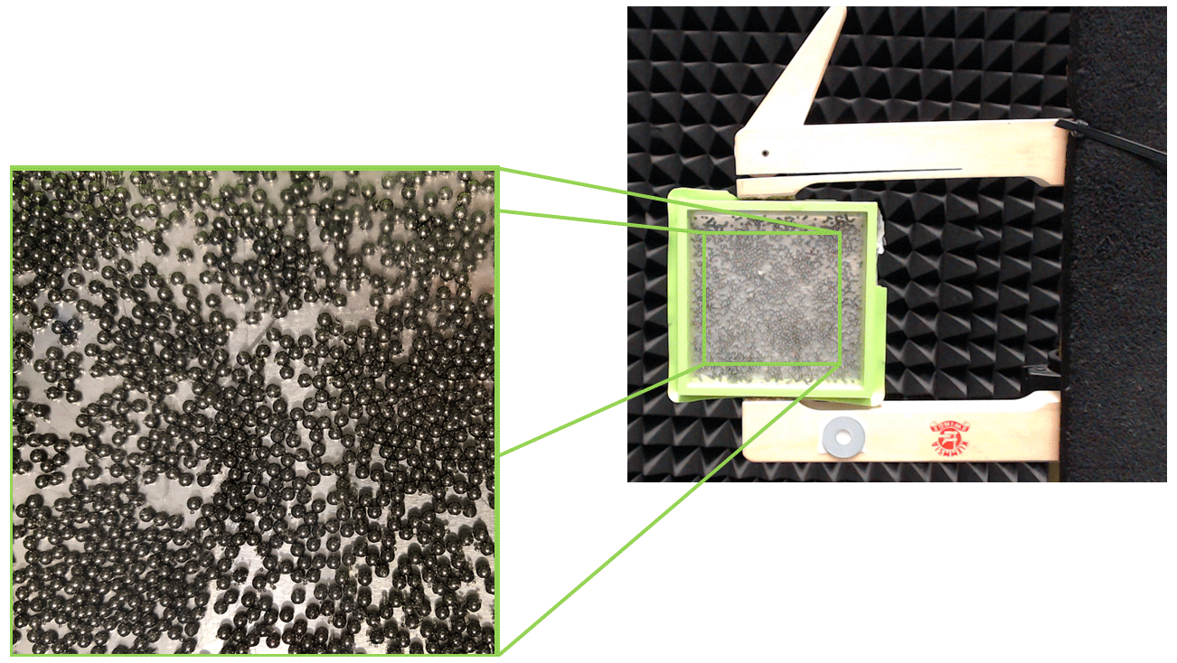
Figure 4Reference sample consisting of an aluminum plate, 1442 bearing balls with a diameter of 2 mm, and a plastic frame as a casting mold mounted in the measurement setup with the reference washer on the mount.
This leaves a missing reference sample for the asymmetric Weibull function. Rinne (2020) presents the Weibull distribution used for describing the grinding of material. So, it was assumed that an irregular surface with scatterers of different sizes, consisting of completely reflecting material, should show such a behavior. Therefore, the second reference probe is generated by crumpling aluminum foil around a piece of styrofoam, which can be seen in Fig. 5. Styrofoam is not visible for the radar sensor, which only leaves the aluminum surface for measurement, which would be perfectly reflecting back to the antenna if mounted as a plain surface. However, the foil is crumpled. Therefore, the sample has a rough surface with irregularities of various sizes. Nevertheless, these irregularities are not distributed randomly, as the crumpling is done in one direction and therefore repeating.
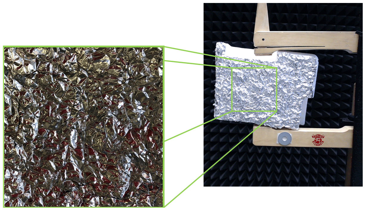
Figure 5Reference sample consisting of a piece of styrofoam surrounded by crumpled aluminum foil, mounted in the measurement setup with the reference washer on the mount.
3.2 Concrete samples
In cooperation with Peter Holzner Bauunternehmen GmbH & Co. KG, a leading construction company in the field of concrete paving and surfaces, two concrete samples with the surfaces structured as available on German roads. The material composition of both samples is the same, which is decreed by the DIN norm for Concrete, reinforced, and prestressed concrete structures – Part 2 (DIN 1045-2:2008-08, 2008). At first, this is a German standard, but is harmonized with Eurocode, what makes it valid all over Europe. The procedure and practical implementation to fulfill this norm is described in detail by Biscoping and Kampen (2017). To cover the differences in processing, two different samples are manufactured. The first one is a sample with a surface structured manually by using a broom finish technique resulting in very well visible grooves. The second sample has a machine-made surface. To be precise, this is a broom finish structure as well, but with distinctly minor grooves and, therefore, a plainer surface. In the former publication, it was referenced as installed as factory made concrete plate. In a real-world implementation, an exactly constant material condition can not be assured due to time variances in surface structuring, material variances, like sand composition and climatic fluctuation. To simulate this effort, structuring hand-crafted surfaces is a common strategy. The structure of the samples is shown in Fig. 6.
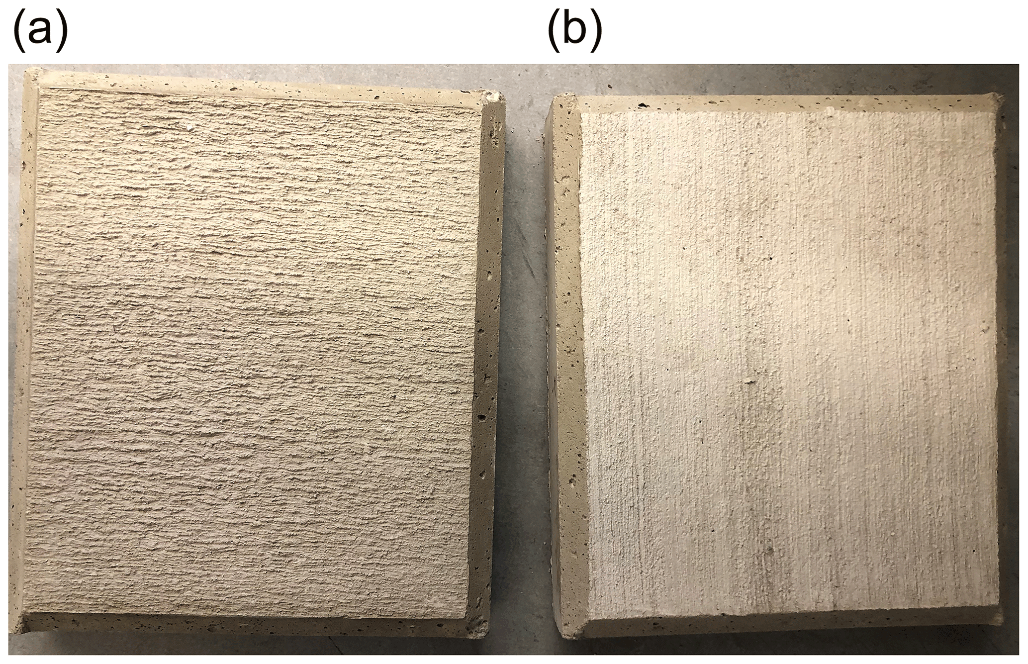
Figure 6Concrete samples for the measurement. (a) Surface structured using a broom finish technique; (b) surface machine-made, resulting in a finer broom finish structure.
In the following section, the measurement results are presented. The complete measurement results of the asphalt surfaces have already been shown in Kurz et al. (2021) and Kurz and Biebl (2022) and are thus only used for comparison but not depicted in total again.
4.1 Reference samples
The SAR image of the reference sample consisting of the bear ball distribution is shown in Fig. 7. An evaluation of the maxima in the area of interest marked by the red rectangle records an attenuation of 8.6 dB. Thus, the attenuation is not exactly the same as measured by the focus-beam setup, but accurate enough. The small variations might come from the not perfectly smooth surface structure of the epoxy resin. Furthermore, one can see some interferences at the edges. Even though the mount can be seen, interference to the especially analyzed area in the red box should be excluded, as the sample juts out of the mount. The SAR image of the other reference consisting of aluminum foil can be seen in Fig. 8. One can see some small local maxima, which probably come from interference due to the material's structure. Else, the SAR image shows a periodically nonuniform surface as desired.
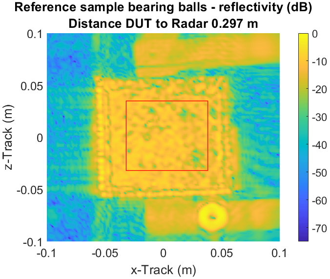
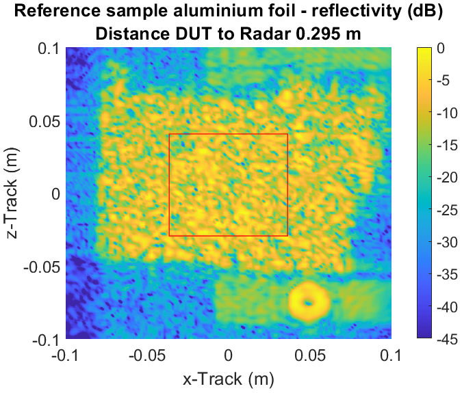
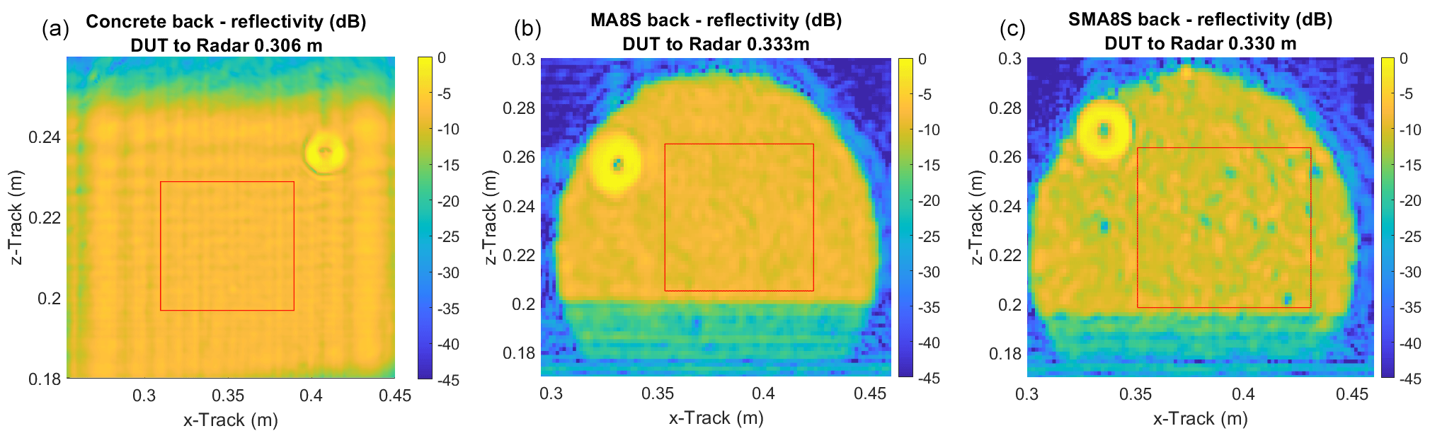
Figure 9Comparison of the reflectivity by material with previous measurements (b, c) already presented in Kurz et al. (2021).
4.2 Concrete samples
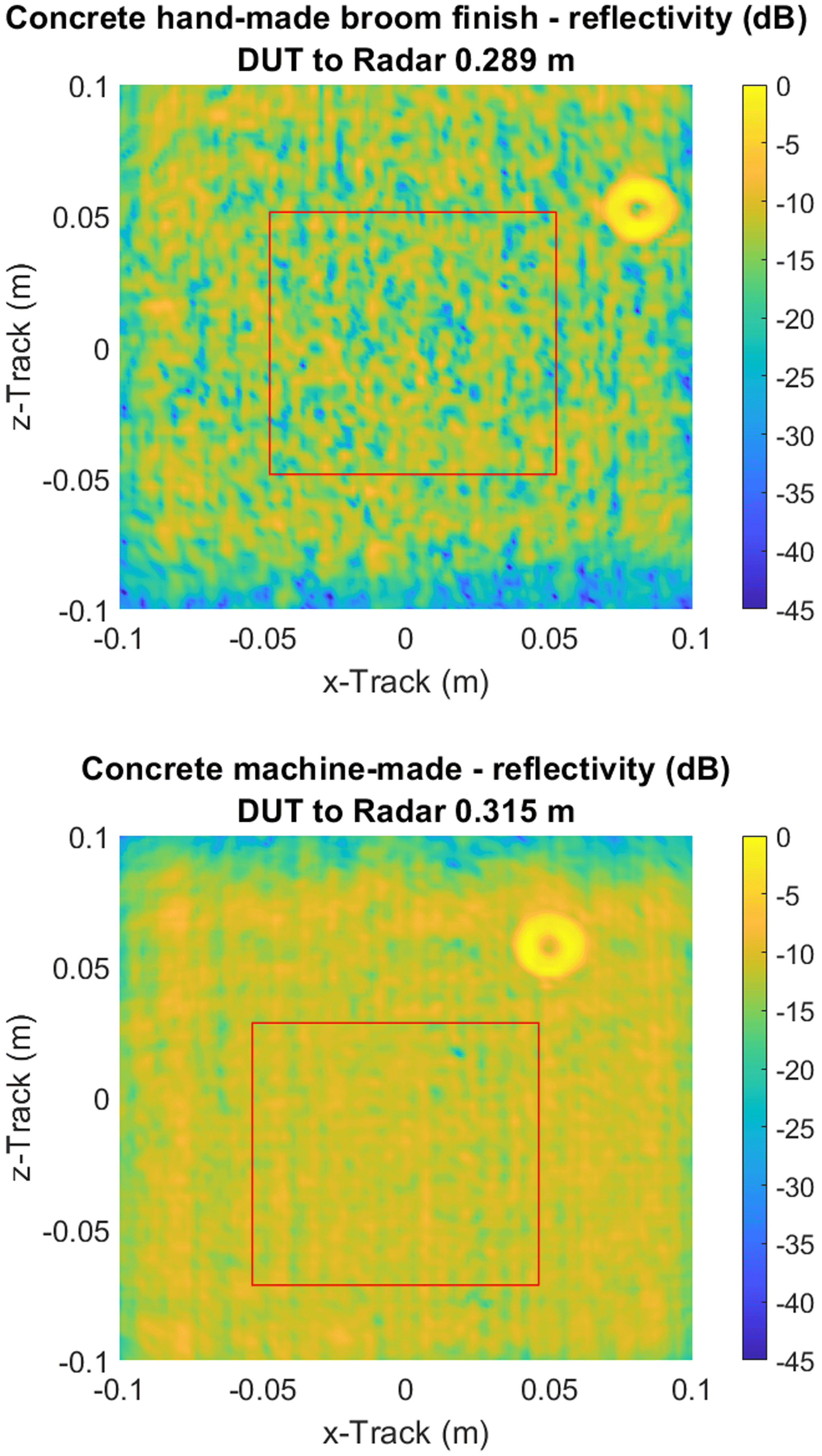
As mentioned in Sect. 3.2 the concrete samples do not differ in material composition from one another. Therefore, a measurement of the rear sides doesn't show any difference. Certainly, a comparison with other road surfaces is of interest, why the results are compared with the results obtained before and presented in Kurz et al. (2021). This is illustrated in Fig. 9. As one can see, the reflectivity slightly differs, especially in the distributed pattern of the reflectivity. Analog to the analysis of the asphalt drill cores from 2021, a difference in relation to the surface structure can be seen as well. The recorded images are shown in Fig. 10. The deeper the grooves, the more variation in reflectivity can be observed. While for flatter grooves like on the bottom figure of Fig. 10, the structure of the reflectivity pattern matches the structure of the grooves, the reflectivity of the handcrafted sample is more irregular due to the rougher surface. In general, the reflectivity of a structured surface like in Fig. 10 is less than for a plain concrete surface like in Fig. 9, and it decreases with increasing roughness. This can be seen as well by comparing the SAR images of concrete with the asphalt ones from Kurz et al. (2021). The reflectivity of the concrete sample with the roughest surface resembles the asphalt samples with the lesser roughness. Once more, the measurements show that the radar reflectivity of common roads for low incidence angles mainly depends on the surface structure and not on the material composition.
So far, all results are qualitative observations. In order to analyze the reflectivity in a more accurate way, its distributions of the amplitude reflection are illustrated in histograms. Therefore, a section of the measurement data, where no edge effects might influence the result, is extracted. This section is marked with a red rectangle in the previous plots. To describe the distributions mathematically, probability density functions are fitted over this data. In the following two types of probability density functions are used, defined in Forbes et al. (2011). At first, the most common distribution, the normal distribution, is defined in Eq. (1)
where μ is the mean and σ2 the variance value. As some of the histograms show a rather asymmetric distribution, a second distribution is necessary. Before, a Weibull distribution was used, as it is commonly used for radar point cloud characterization. Now, we use a special case of the Weibull distribution, the Rayleigh distribution. A Weibull distribution with a shape factor k of two is a Rayleigh distribution (Kottegoda, 2008, p. 209). As this distribution fits all corresponding data sets as well, the Rayleigh distribution with only one degree of freedom, being the scale factor λ is preferable. It is defined in Eq. (2).
5.1 Validation of the measurement setup
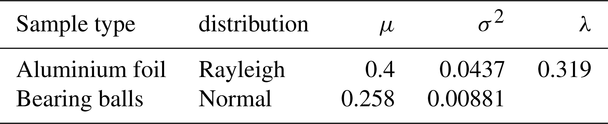
At first, the measurements of the reference samples are further analyzed. The resulting histograms are depicted in Fig. 11, and the corresponding parameter values are listed in Table 1. As assumed initially, one can see that the reflectivity behavior of the reference sample consisting of crumpled aluminum foil can be fitted fine using a Rayleigh distribution. Likewise it confirms that the reflectivity behavior of the reference sample consisting of the randomly distributed bearing balls on an aluminum plate can be fitted properly using a normal distribution. Thus, the measurement approach and setup, as well as the post-processing, is verified.
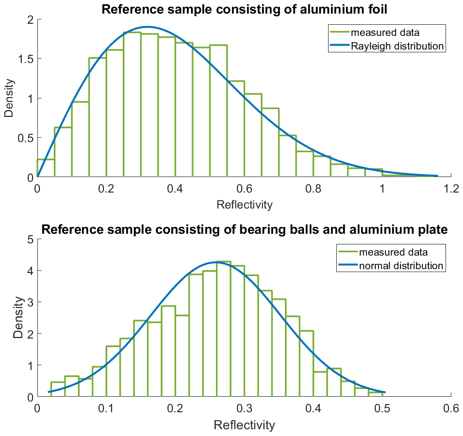
Figure 11Histograms of the reflectivity for the reference sample consisting of crumpled aluminum foil on the top and for the reference sample consisting of the randomly distributed bearing balls on an aluminum plate, both fitted with a probability density distribution function.
Table 1Parameter of the distribution fits, the corresponding mean μ and variance σ2 values for both reference samples.
5.2 Alignment of asphalt sample distibutions
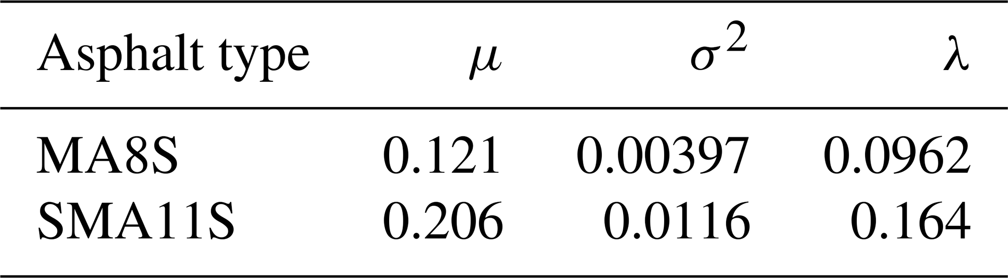
As the validation is done using Rayleigh distribution fits, the histograms presented in Kurz and Biebl (2022, p. 4) are extended with a Rayleigh distribution fit for better comparison. These asphalt types are mastic asphalt with a maximum grain size of 8 mm (MA8S) and split mastic asphalt with a maximum grain size of 11 mm (SMA11S). The resulting graphs are depicted in Fig. 12, and the corresponding parameters are listed in Table 2. For MA8S, Weibull and Rayleigh distribution are the same, as they should be by definition. For SMA11S, the shape factor was only approximately two (k=1.97). Therefore, they do not lie exactly on top of each other but are very similar. The scale factor λ changes from 0.232 to 0.164. Mean stays with μ=0.205 the same, while the variance σ2 changes slightly from 0.0119 to 0.0115.
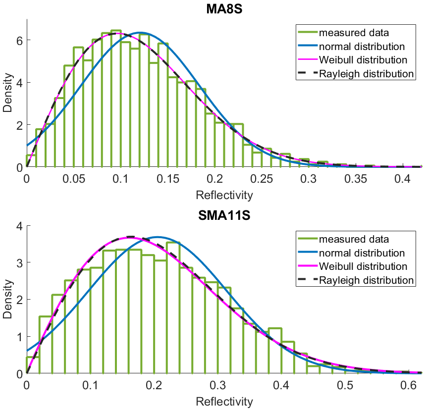
Figure 12Histograms of the reflectivity for the Weibull fit asphalts presented by Kurz and Biebl (2022, p. 4) extended with a Rayleigh distribution fit.
Table 2Scale parameter of the Rayleigh distribution fits and the corresponding mean μ and variance σ2 values for both asphalt measurements.
5.3 Concrete samples
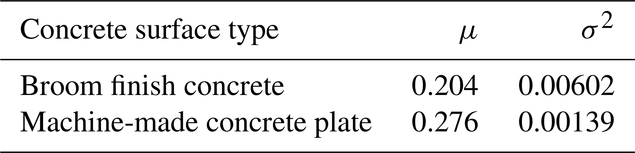
The same fitting is finally done for the measurement of the concrete surfaces. Figure 13 shows the fitted data on the top for the broom finish sample and on the bottom for the machine-made concrete plate. The reflectivity for both samples can be described using a normal distribution fit varying in mean and variance. The corresponding mean and variance values are summarized in Table 3.
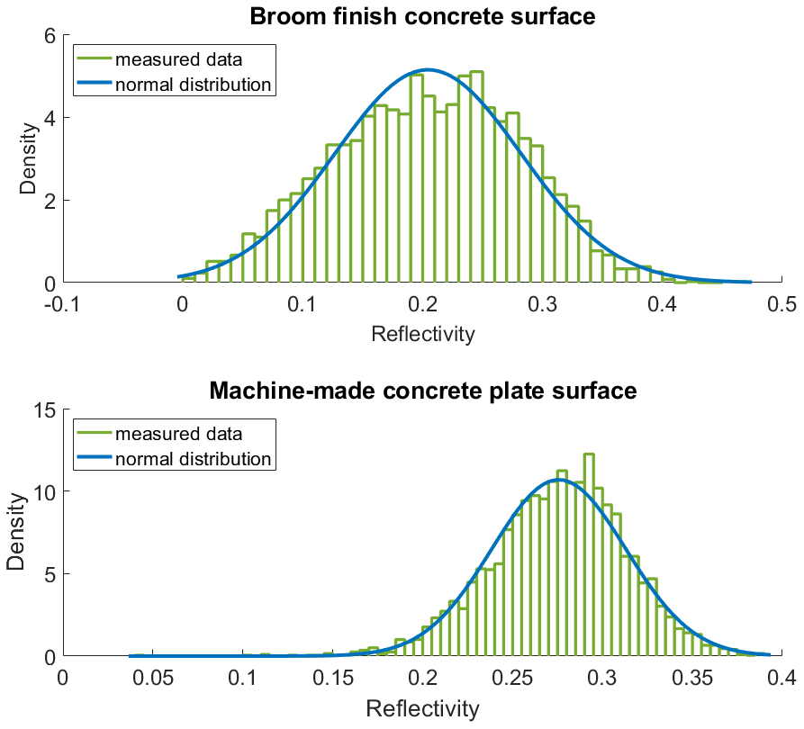
Figure 13Histograms of the reflectivity of broom finish concrete on the top and a machine-made concrete plate on the bottom, both fitted using a normal probability density function.
Table 3Mean μ and variance σ2 values for both concrete sample measurements.
Here, a SAR setup to measure the reflectivity of road surfaces in a laboratory environment is shown. This setup is validated, and the reflectivity of roads built of concrete is determined using two samples representing the extrema in concrete manufacturing on roads. Processing the resulting SAR images leads to probability density functions, characterizing the scattering of concrete on roads. A comparison with formerly shown measurements of asphalt on roads is drawn. The work completes the former studies on radar reflectivity and scattering on the most common German highway surfaces.
The research data used in this paper can be requested from the authors.
VK, MF, and FP developed the measurement setup for the laboratory measurements. VK determined and organized the samples. VK generated the references. VK and MF performed the SAR measurements. FP performed the focus-beam measurement. VK and MF post-processed the obtained data, and VK prepared the manuscript. All other authors gave feedback and approved the final version. EB supervised the project.
The contact author has declared that none of the authors has any competing interests.
Publisher’s note: Copernicus Publications remains neutral with regard to jurisdictional claims in published maps and institutional affiliations.
This article is part of the special issue “Kleinheubacher Berichte 2022”. It is a result of the Kleinheubacher Tagung 2022, Miltenberg, Germany, 27–29 September 2022.
The study of the asphalt drill cores was done in cooperation with the Centre for Building Materials of the Technical University of Munich. Special thanks again for providing the samples. The work on concrete was done in cooperation with Peter Holzner Bauunternehmen GmbH & Co. KG. Special thanks to them for providing the concrete samples and especially to Thomas Wandinger and Florian Rampfl for the technical support.
This paper was edited by Jens Anders and reviewed by two anonymous referees.
Babu, A. and Baumgartner, S. V.: Road Surface Quality Assessment Using Polarimetric Airborne SAR, 2020 IEEE Radar Conference (RadarConf20), 21–25 September 2020, Florence, Italy, IEEE, https://doi.org/10.1109/RadarConf2043947.2020.9266588, 2020. a
Biscoping, M. and Kampen, R.: Zusammensetzung von Normalbeton – Mischungsberechnung, InformationsZentrum Beton GmbH, https://mitglieder.vdz-online.de/fileadmin/gruppen/vdz/3LiteraturRecherche/Zementmerkblaetter/ZM_B20_2017_2.pdf (last access: 21 January 2023), 2017. a
DIN 1045-2:2008-08: Tragwerke aus Beton, Stahlbeton und Spannbeton – Teil 2: Beton – Festlegung, Eigenschaften, Herstellung und Konformität – Anwendungsregeln zu DIN EN 206-1, Beuth Verlag GmbH, https://doi.org/10.31030/1453177, 2008. a
Forbes, C. S., Evans, M., Hastings, N. A. J., and Peacock, B.: Statistical distributions, 4th edn., Wiley, Hoboken, New Jersey, USA, ISBN 9780470627235, 2011. a, b
Henry, C., Azimi, S. M., and Merkle, N.: Road Segmentation in SAR Satellite Images With Deep Fully Convolutional Neural Networks, IEEE Geosci. Remote S., 15, 1867–1871, https://doi.org/10.1109/LGRS.2018.2864342, 2018. a
Hirsenkorn, N., Subkowski, P., Hanke, T., Schaermann, A., Rauch, A., Rasshofer, R., and Biebl, E.: A ray launching approach for modeling an FMCW radar system, 2017 18th International Radar Symposium (IRS), 28–30 June 2017, Prague, Czech Republic, IEEE, https://doi.org/10.23919/IRS.2017.8008120, 2017. a
Kottegoda, N. T.: Applied statistics for civil and environmental engineers, 2nd edn., Blackwell Pub, Oxford, UK, ISBN 9781444309416, 2008. a
Kurz, V. and Biebl, E.: MmWave Scattering Properties of Objects in Automotive Scenarios, in: 2022 Kleinheubach Conference, 27–29 September 2022, Miltenberg, Germany, IEEE, 1–4, ISBN 978-3-948571-07-8, 2022. a, b, c, d
Kurz, V., Stuelzebach, H., Pfeiffer, F., van Driesten, C., and Biebl, E.: Road Surface Characteristics for the Automotive 77 GHz Band, Adv. Radio Sci., 19, 165–172, https://doi.org/10.5194/ars-19-165-2021, 2021. a, b, c, d, e, f, g
Li, E. S. and Sarabandi, K.: Low grazing incidence millimeter-wave scattering models and measurements for various road surfaces, IEEE T. Antenn. Propag., 47, 851–861, https://doi.org/10.1109/8.774140, 1999. a
Mahapatra, D. K., Pradhan, K. R., and Roy, L. P.: An experiment on MSTAR data for CFAR detection in lognormal and weibull distributed sar clutter, in: 2015 International Conference on Microwave, Optical and Communication Engineering (ICMOCE), 19–20 December 2015, Bhubaneswar, India, IEEE, 377–380, https://doi.org/10.1109/ICMOCE.2015.7489771, 2015. a
Pfeiffer, F., Biebl, E., and Siedersberger, K.-H.: Determination of Complex Permittivity of LRR Radome Materials Using a Scalar Quasi-Optical Measurement System, Springer Berlin Heidelberg, Berlin, Heidelberg, 205–210, https://doi.org/10.1007/978-3-540-77980-3_16, 2008. a
Rinne, H.: The Weibull distribution: A handbook, Chapman & Hall/CRC, Boca Raton, ISBN 9780367577469, 2020. a
Schneider, R., Didascalou, D., and Wiesbeck, W.: Impact of Road Surfaces on Millimeter-WavePropagation, IEEE T. Veh. Technol., 49, 1314–1320, https://doi.org/10.1109/25.875249, 2000. a
Wald, S. O. and Weinmann, F.: Ray Tracing for Range-Doppler Simulation of 77 GHz Automotive Scenarios, 2019 13th European Conference on Antennas and Propagation (EuCAP), 31 March–5 April 2019, Krakow, Poland, IEEE, ISBN`978-1-5386-8127-5, 2019. a
Winner, H.: Introducing autonomous driving: an overview of safety challenges and market introduction strategies, at – Autom., 66, 100–106, https://doi.org/10.1515/auto-2017-0106, 2018. a