AI Models for Supporting SI Analysis on PCB Net Structures: Comparing Linear and Non-Linear Data Sources

Signal integrity (SI) is an essential part in assuring the functionality of microelectronic components on a printed circuit board (PCB). Depending on the complexity of the designed interconnect structure, even the experienced PCB developer might be reliant on multiple design cycles to optimally configure the PCB parameters, which eventually results in a very complex, time-consuming and costly process. Under these aggravating conditions, artificial intelligence (AI) models may have the potential to support and simplify the SI-aware PCB design process by building predictive models and proposing design solutions to streamline the existing workflows and unburden the PCB designer. In this paper, the AI approach is divided into two separate stages consisting of neural network (NN) regression in the first step and parameterization of the PCB net structure in the second step. First, the NN models are applied to learn the relationship between the electrical parameters and the resulting signal quality captured by domain-oriented signal features in the time domain. Second, based on the trained NN models, on the one hand, the k-nearest neighbor (kNN) method is utilized to select solution candidates within the feature space, while on the other hand, genetic algorithms (GA) are applied to directly optimize the parameters of the interconnect structure. Moreover, the influence of the simulation abstraction level is investigated by comparing simulation data originating from linear and I/O buffer information specification (IBIS)-based non-linear modeling of the integrated circuit (IC) characteristics concerning the prediction accuracy and direct transferability. Finally, transfer learning concepts are evaluated to exchange learned knowledge representations between the different modeling of the IC characteristics to improve data efficiency and reduce computational complexity.

1 Introduction

The various stages of the design of printed circuit boards (PCB) as well as system integration and handling of physical couplings are addressed by the different engineers involved. In this context, ensuring signal integrity (SI) is an integral part to comply with functional and electromagnetic compatibility (EMC) design constraints at PCB level. For designers who have little to no experience with SI trying to fulfill these design constraints is challenging and error-prone.

Artificial intelligence (AI) models may serve as a possible reference during the PCB design process for designers working on the selection of the routing structure in the pre-layout phase. These models are intended to assist them in specifying signal topologies and routing structures that will affect the SI of the system. For the realization of AI models, an extension has to be made with respect to AI-specific data sources and objects based on a generalized design process for electronic systems. In the future, AI-supported pre-layout measures will be used in the specification and design phases. For this purpose, e.g. for the development of an SI concept for upcoming design tasks, the generalized PCB design process presented in John et al. (2022) and the extended combined process and phase model presented in Ecik et al. (2023) are essential. The generalized approach for the integration of AI models into the PCB design process is illustrated in Fig. 1 demonstrating how different AI models might be utilized and combined to support SI-compliant design decisions. Therefore, the integration of domain knowledge from experienced PCB developers is of utmost importance to detect adequate design solutions, support the unexperienced developer and effectively reduce the number of design cycles.

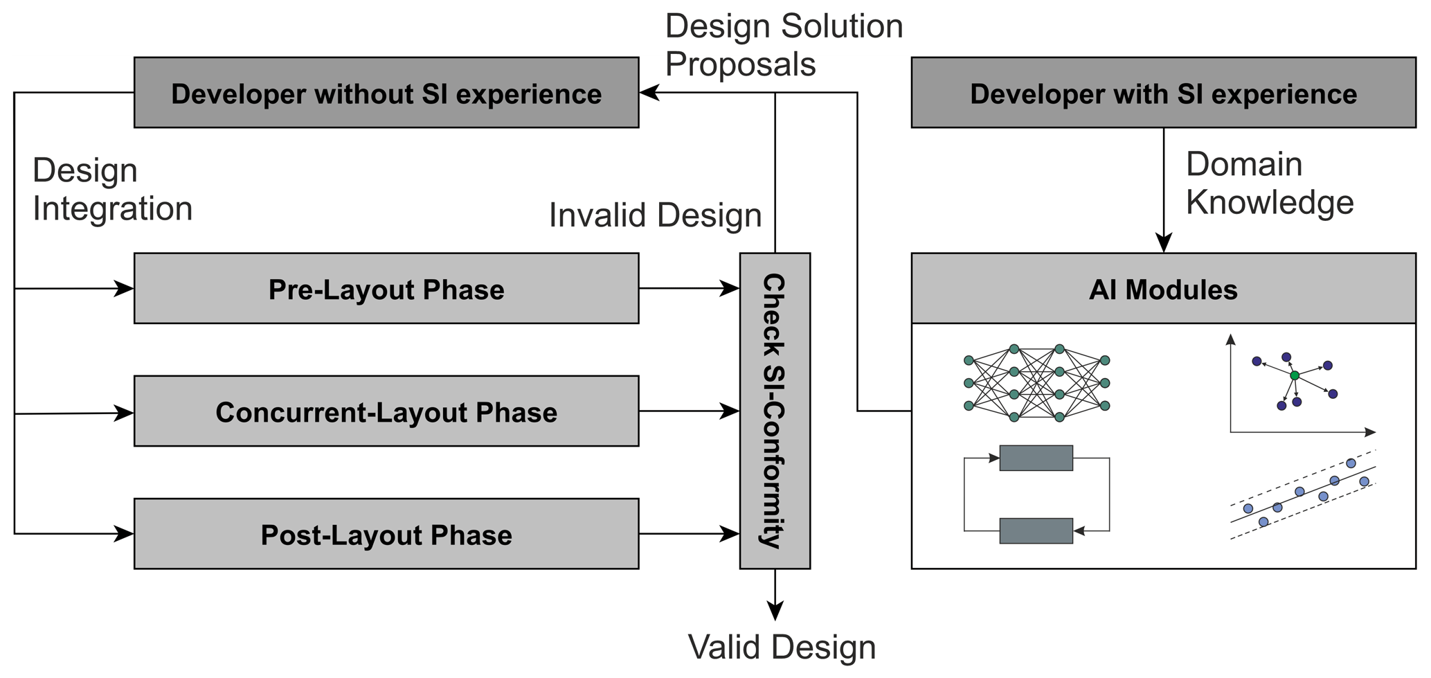
Figure 1 Illustration of the generalized procedure to integrate AI-based SI design support into the PCB design process with consideration of domain knowledge from the experienced SI developer.

Recently, AI or in particular methods from the machine learning (ML) subdomain have received growing attention in the realm of electronic design automation (EDA) and PCB design under SI constraints. Most prominently the prediction and optimization of eye diagram parameters such as eye height and eye width from parameters of the transmitter, interconnect and receiver has been a main research focus. In Lu et al. (2018) support vector regression (SVR) and neural network (NN) ML methods were utilized to predict the eye diagram parameters from the specified PCB parameters. Originating from this initial publication several improvements with respect to the ML implementations have been achieved. With respect to the SVR, an active-subspace method has been proposed in Ma et al. (2020a, b) to improve the algorithmic performance. Regarding the NN, methods to improve the data efficiency such as transfer learning in Zhang et al. (2019) and semi-supervised learning in Chen et al. (2020) have been deployed.

The inverse problem setting, which initializes with the target eye performance to find the required electrical parameters, was firstly discussed in the prospect on future work section of Lu et al. (2018). In Trinchero et al. (2019) and Roy et al. (2019) this inverse design was addressed similarly to the forward model by directly applying SVR and NN regression approaches, respectively. The inverse problem formulation however, is intrinsically ill-posed as ambiguities and one-to-many mappings result from the physical relationships leading to non-unique solutions and inaccuracies in the predictions. Therefore, procedures to include the forward model into the inverse regression problem formulation have been recently developed by Ma et al. (2022), where tandem NNs are used to integrate the forward model into the process to improve the inverse predictions.

Alternatively, Kim et al. (2018) and Zhang et al. (2022) suggested to remain solely with the forward NN model and then applying an optimization method such as a genetic algorithm (GA) based on this model to find an optimal solution. However, the simplifying usage of the forward model has to be compensated by the additional computational complexity induced by the utilization of an optimization algorithm.

2 Methodology

In this paper, we present a different approach compared to the eye diagram-based applications that are widely used in the literature. Extraction of specific signal descriptive time domain features enables SI analysis and design support during the PCB layout phases. Various common PCB net structures can be investigated using this generic approach, see John et al. (2022). Furthermore, a two-stage AI framework is established. During the first step, NN regression models are implemented to learn the relationship between the electrical PCB parameters and the defined signal time domain features in both, forward and inverse direction. Then, during the second step, the learned representations stored in the NN models are utilized to parameterize the interconnect structure and provide design suggestions. In this context, the k-nearest neighbor (kNN) algorithm is applied as a feature-based pre-selection method to find solution candidates within a feature space population as input for the inverse NN model, while the GA optimizes the PCB parameters directly based on the forward NN model.

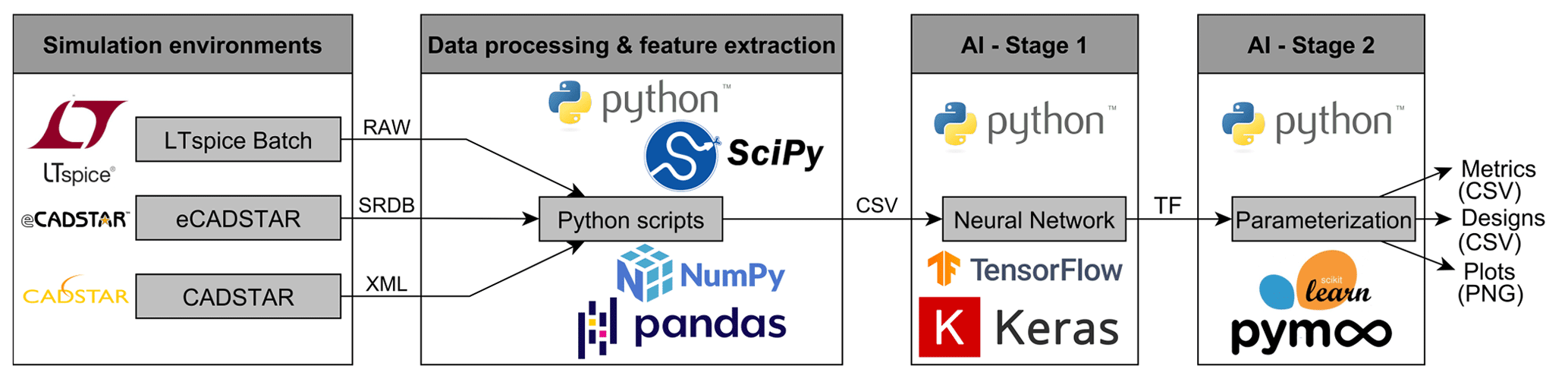
Figure 2 Illustration of the underlying toolchain and data flow of the proposed approach. The two elements on the left represent the provision of learning data, while the two elements on the right show the two-stage AI framework.

Figure 2 provides an overview of the underlying toolchain and data flow of the proposed methodology. This includes the simulation environment for data generation, the data processing and feature extraction to provide learning datasets and finally the two-stage AI framework. The utilized simulation environments are LTspice (see Analog Devices, 2021) and CADSTAR/eCADSTAR (see Zuken, 2021a, b), with only the latter two capable of reasonably translating I/O buffer information specification (IBIS) models for non-linear integrated circuit (IC) characteristics, while LTspice is limited to linear IC modeling. The simulation data is then further processed and the time-domain features are extracted within Python to generate learning datasets. These features are defined by:

$$\begin{array}{}\text{(1)}& E_{\mathrm{c}}=\underset{-\mathrm{\infty }}{\overset{\mathrm{\infty }}{\int }}\left|V\right(t{)}^{\mathrm{2}}|\mathrm{d}t<\mathrm{\infty }{E}_{\mathrm{d}}=\sum _{i=\mathrm{1}}^J|V_i\left(t{)}^{\mathrm{2}}\right|(t_i-t_{i-\mathrm{1}})\end{array}$$

$$\begin{array}{}\text{(2)}& H=-\sum _{k\in K}{p}_k{\log }_{\mathrm{2}}{p}_k{H}_{\mathrm{scaled}}={\displaystyle \frac{H}{H_{\max }}}={\displaystyle \frac{H}{{\log }_{\mathrm{2}}K}}\end{array}$$

$$\begin{array}{}\text{(3)}& \mathrm{SR}={\displaystyle \frac{V_{\mathrm{90}\mathit{\%}}-V_{\mathrm{10}\mathit{\%}}}{t_{\mathrm{r}}}}={\displaystyle \frac{V_{\mathrm{90}\mathit{\%}}-V_{\mathrm{10}\mathit{\%}}}{t\left(V_{\mathrm{90}\mathit{\%}}\right)-t\left(V_{\mathrm{10}\mathit{\%}}\right)}}\end{array}$$

$$\begin{array}{}\text{(4)}& V_{\max }=max\left(V\right)\end{array}$$

where E_d, H_scaled, SR and V_max correspond to discrete energy, scaled entropy, slew rate and maximum voltage, respectively. Also, the variable J is associated with the number of voltage samples and K with the number of unique voltage samples, while the variable p_k is equivalent to the voltage amplitude probability density. The created learning datasets are then applied to the two-stage AI framework in the next step. In this context, the NN architectures are built with the Keras library (Chollet, 2015), which is embedded into the Tensorflow framework (Abadi et al., 2015), while the kNN algorithms are implemented using the scikit-learn library (Pedregosa et al., 2011) and the GA is derived from the pymoo library (Blank and Deb, 2020).

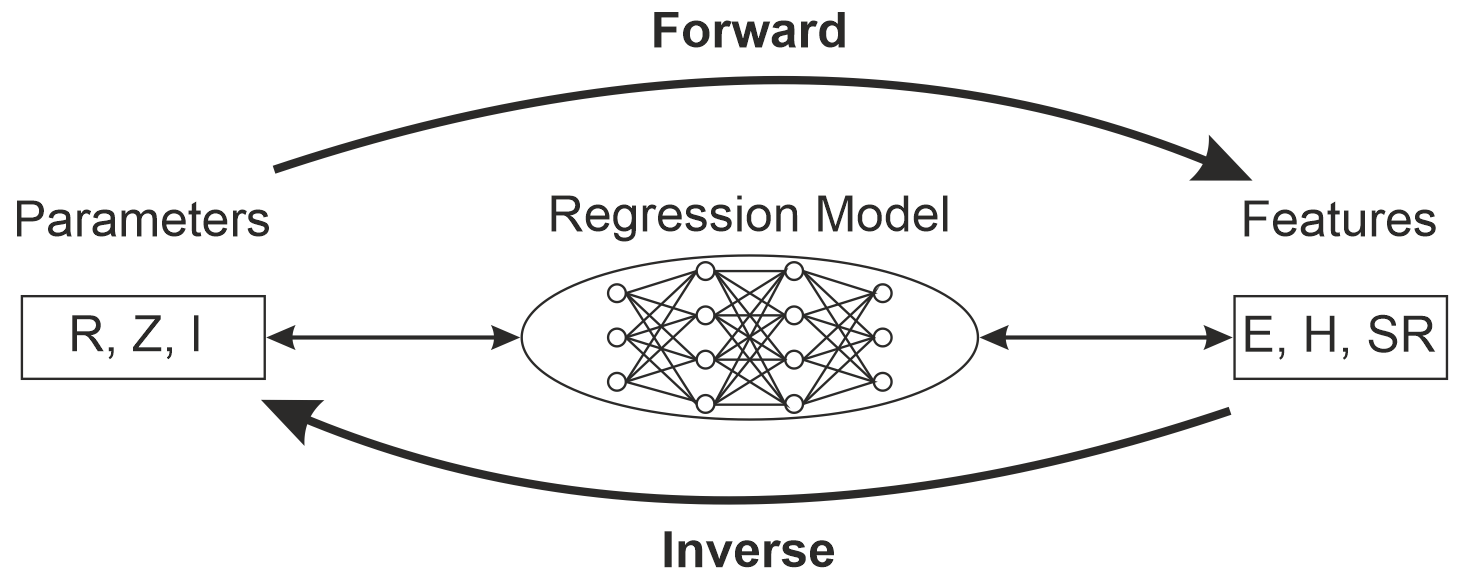
Figure 3 Illustration of the forward and inverse mode regression. Forward mode regression corresponds to the prediction of features from given electrical parameters, while inverse mode regression represents the direct opposite i.e. the prediction of electrical parameters from given features.

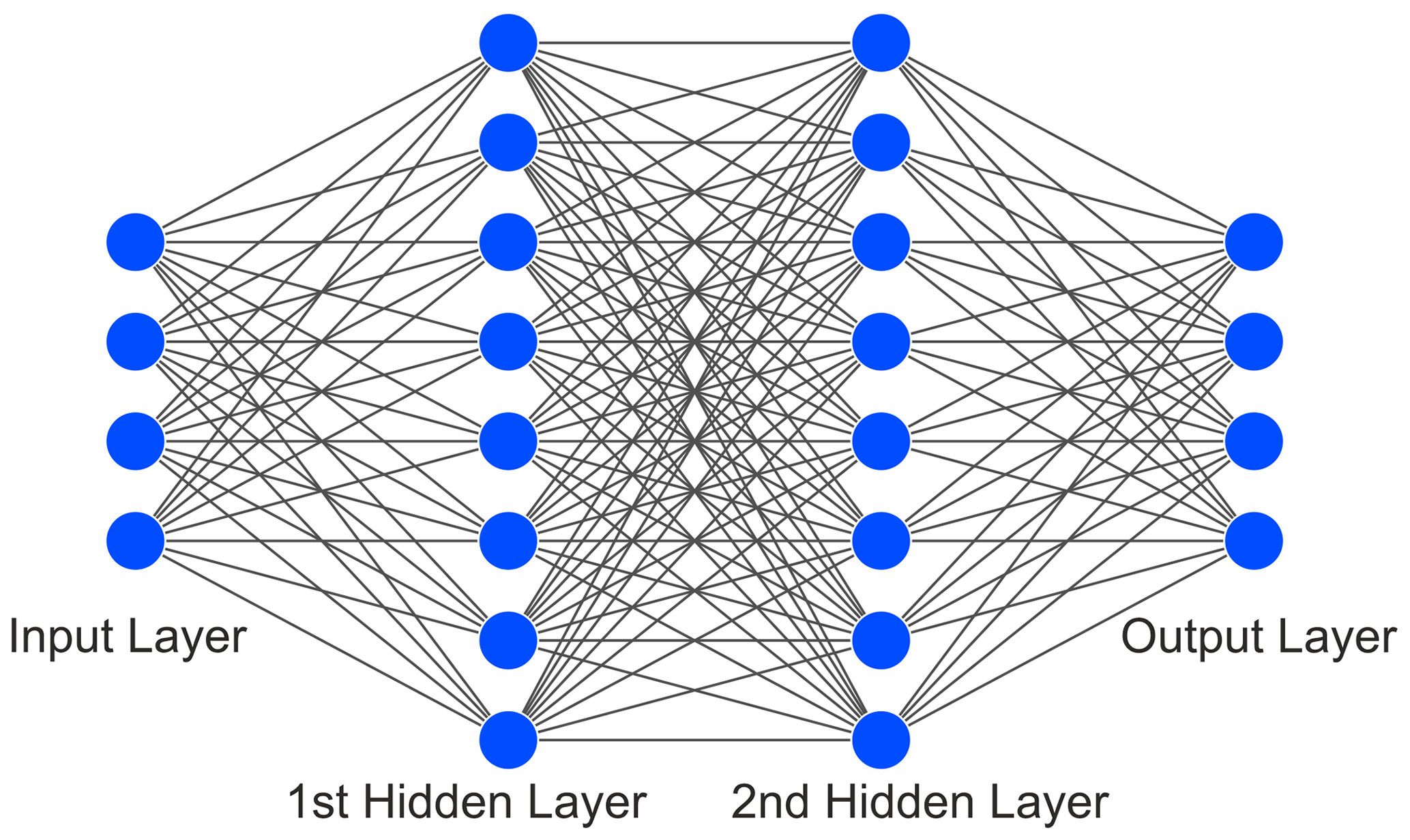
Figure 4 Illustration of the structure of the implemented NN architecture with input, output and two hidden layers.

3 Machine Learning Methods

The most important element of the AI framework are the NN architectures. NNs have been proven to be a suitable tool for regression tasks to support SI analysis, see Lu et al. (2018) and Roy et al. (2019). The implemented NN regression models realize the prediction of numeric values either in forward or inverse mode as shown in Fig. 3. The structure of the utilized NN is depicted in Fig. 4 consisting of input, output and two hidden layers, each with a specified number of neurons, which hold an adjustable weight and an activation function. During the training of the NN a certain amount of data examples corresponding to the batch size are inserted in the input layer and propagated through the network with its current weights to finally compute the loss at the output layer. For the implemented regression this loss is equivalent to the mean squared error (MSE) loss:

$$\begin{array}{}\text{(5)}& \mathrm{MSE}={\displaystyle \frac{\mathrm{1}}{N}}\sum _{i=\mathrm{1}}^N(\widehat{y_i}-y_i{)}^{\mathrm{2}}\end{array}$$

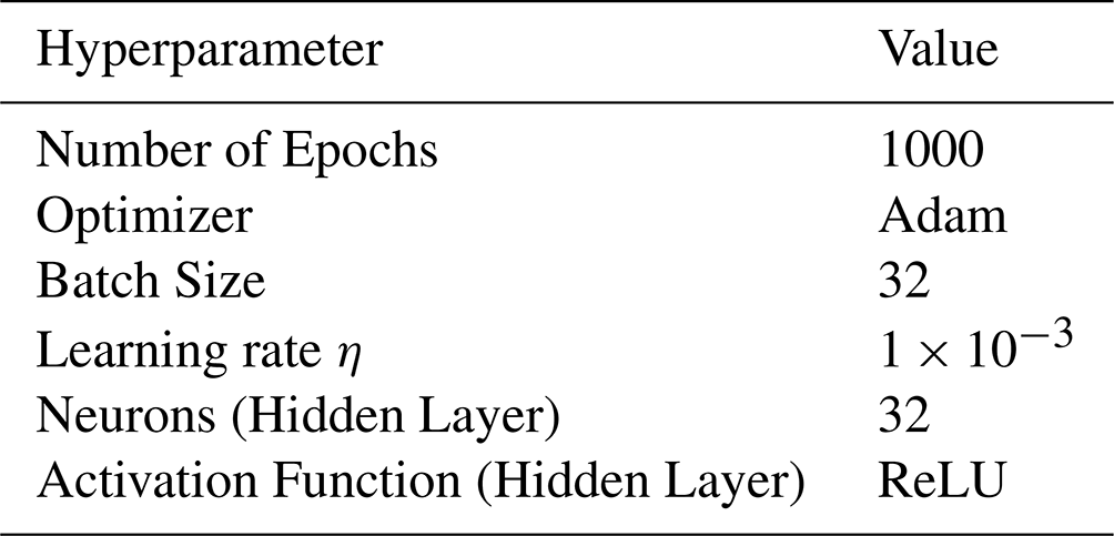
where N, y_i and $\widehat{y_i}$ are associated with the number of data examples, true value and predicted value, respectively. The loss is then iteratively minimized by adjusting the neuron weights using backpropagation and automatic differentiation principles in the individual training steps also known as epochs. For further information on the fundamentals of NNs, see Goodfellow et al. (2016). Finally, this results in a number of NN hyperparameters, which are summarized in Table 1 for the implemented NN.

Important metrics for the evaluation of the regression performance are the root mean squared error (RMSE), which is determined by extracting the root from the MSE of Eq. (5), to measure the actual occurring prediction deviations in the same order of magnitude as the observed variable and the R²-Score as defined by:

$$\begin{array}{}\text{(6)}& R^{\mathrm{2}}={\displaystyle \frac{{\sum }_{i=\mathrm{1}}^N(\widehat{y_i}-\stackrel{\mathrm{‾}}{y_i}{)}^{\mathrm{2}}}{{\sum }_{i=\mathrm{1}}^N(y_i-\stackrel{\mathrm{‾}}{y_i}{)}^{\mathrm{2}}}}=\mathrm{1}-{\displaystyle \frac{{\sum }_{i=\mathrm{1}}^N(y_i-\widehat{y_i}{)}^{\mathrm{2}}}{{\sum }_{i=\mathrm{1}}^N(y_i-\stackrel{\mathrm{‾}}{y_i}{)}^{\mathrm{2}}}}\end{array}$$

denoting the explainability of the regression, where $\stackrel{\mathrm{‾}}{y_i}$ is associated with the mean true value.

To ensure the performance and convergence of the NN, prior to the training, the input data x and output data y is normalized according to:

$$\begin{array}{}\text{(7)}& x_{\mathrm{norm}.}={\displaystyle \frac{x-x_{\min }}{x_{\max }-x_{\min }}}{y}_{\mathrm{norm}.}={\displaystyle \frac{y-y_{\min }}{y_{\max }-y_{\min }}}\end{array}$$

Table 1 Hyperparameter setting of the NN.

Also, the dataset is split into 70 % training, 20 % validation and 10 % testing data. The NN model is exclusively exposed to the training data for the learning process, while the validation data is simultaneously utilized to evaluate the performance on unseen data. The testing data is not employed before the training of the model is completed and is then utilized to evaluate the performance on data that has not been considered during the whole training process.

Table 2 List of BO-tunable hyperparameters and their lower and upper tuning limits. Note that each of the hidden layer hyperparameters are individually tuned. The additional hyperparameter dropout factor realizes a regularization by randomly ignoring a defined percentage of neurons during each training epoch.

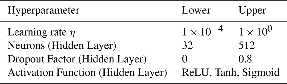
In addition to the default hyperparameter configuration denoted in Table 1, another configuration based on Bayesian optimization (BO) for hyperparameter tuning is realized. The tuning with BO is based on an underlying Gaussian process regression, which models the MSE loss as the objective function with the NN hyperparameters as input variables, which is iteratively minimized by taking previous evaluations into consideration. For further insights on BO, see Frazier (2018). The mentioned properties render BO to be superior in terms of efficiency especially for high-dimensional hyperparameter spaces compared to random or grid search, which roam the hyperparameter space more blindly and are not equipped with any form of memory of past evaluations. For the implemented BO, 50 iterations are carried out and the tunable hyperparameters with their respective tuning limits are represented in Table 2. The number of epochs and batch size hyperparameters are not tuned to allow a fair comparison to the default configuration.

The implemented kNN algorithm is a basic unsupervised ML method, which can be used for feature-based pre-selection. In collaboration with the inverse NN model this has proven to be a promising approach for SI design support as described in John et al. (2022). kNN is a proximity-based approach that searches k feature sets, which are distance-wise the closest to a given feature example within a feature population sampled from a multivariate normal distribution encompassing the entire feature space. The features are normalized according to Eq. (7) before application. The kNN algorithm is realized with k set to 5 using the Euclidean distance metric and the brute force computation method.

Finally, the GA is a search and optimization procedure belonging to the class of evolutionary algorithms. In combination with the forward NN model, GA methods have proven to be effective in finding optimal SI design solutions as demonstrated in Kim et al. (2018) and Zhang et al. (2022). By definition, the GA optimization is initialized with a randomly sampled population of size M, which iteratively goes through the evolutionary phases of evaluation, selection, crossover and mutation to eventually minimize a given optimization objective. The implemented GA is realized with a population size M of 100 and with Simulated Binary Crossover (SBX), see Deb et al. (2007). For further information on the underlying GA principles, see Goldberg (1989) as well as Bäck and Schwefel (1993). For the objective functions of the implemented single-target GA the Mean Absolute Error (MAE) as defined by:

$$\begin{array}{}\text{(8)}& \mathrm{MAE}={\displaystyle \frac{\mathrm{1}}{N}}\sum _{i=\mathrm{1}}^N|\widehat{y_i}-y_i|\end{array}$$

is chosen as the minimization metric. Fundamentally, there are two different objectives for the GA, the most simple and obvious one being the minimization of the MAE distance to a desired pre-defined feature set. This leads to the optimization objective O₁ defined by:

$$\begin{array}{}\text{(9)}& min{O}_{\mathrm{1}}=\mathrm{MAE}(\mathit{F};{\mathit{F}}_{\mathrm{target}}),\end{array}$$

where F is the feature vector computed by the NN forward model and F_target is the desired feature set. Another more implicit approach is the simultaneous minimization or maximization of certain features e.g. in this specific case the maximization of energy and slew rate, while concurrently minimizing entropy and maximum voltage. This problem definition is appropriate from a SI perspective as the desired signal waveforms should have a rather high slew rate and energy to prevent slowly rising signal slopes, while the maximum voltage should be rather low to prevent overshoots. Additionally, the entropy should also be rather low corresponding to signals with less information content, which are more similar to an ideal square wave signal, while high entropy correlates with overshoot or low slew rate signals, both of which are suboptimal. This results in the optimization objective O₂ defined by:

$$\begin{array}{}\text{(10)}& min{O}_{\mathrm{2}}=\mathrm{MAE}\left(\left[\mathrm{1}-E_{\mathrm{d}};H_{\mathrm{scaled}};\mathrm{1}-\mathrm{SR};U_{\max }\right];\mathbf{0}\right),\end{array}$$

Note that in both instances the features are normalized according to Eq. (7).

4 Generation of Simulation Data

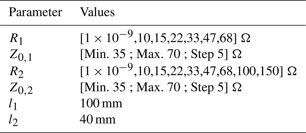
For the training of the AI models data has been generated using the LTspice and the CADSTAR simulation environments based on the far end cluster shown in Fig. 5. The far end cluster operates with a clock frequency of 50 MHz at 3.3 V using the Texas Instruments SN74AC86 IBIS model for driver and receiver. Concerning the transmission lines, routing on inner layers (symmetric stripline) was assumed. A parameter variation as shown in Table 3 was utilized to generate 4032 simulation data samples. Besides the IBIS-based non-linear simulation in CADSTAR two simulation datasets with linear IC characteristics have been created in LTspice and CADSTAR, respectively, where the voltage as well as rise and fall times were adjusted according to the IBIS model.

Table 3 Applied parameter variation. Note that each parameter is varied individually and not simultaneously.

4032 data samples

Following the results presented in John et al. (2022), the parameters for drivers and receivers in AC technology (AC86) used there for linear and IBIS-based non-linear models were also used for this paper. On the one hand, this allows a detailed comparison with the AI procedures and methods discussed in John et al. (2022), and on the other hand, the further use of the database already available there. Furthermore, we expect that in the future complete AC86 SPICE decks will be available for additional investigations in order to be able to carry out additional process tests.

5 Application of the Artificial Intelligence Models

Based on the far end cluster topology defined in Fig. 5, different simulation data sources with linear and non-linear modeling of the IC characteristics were compared concerning the accuracy, applicability and transferability of the trained AI models.

5.1 Neural Networks

NN architectures have been trained in both, the forward and inverse mode, according to Fig. 3. First, the forward NN was investigated, whose regression accuracy in predicting the features from the electrical parameters is shown in Fig. 6. A consistently high regression accuracy was noticeable for each of the observed simulation datasets, which is also reflected in the regression metrics in Table 4 as testing R²-Scores above 99 % and invariably small normalized testing RMSE values below 2 % have been observed. As the default hyperparameter configuration already provides very accurate results, the hyperparameter tuning with BO at most only results in marginal improvements in regression performance.

Figure 5 Schematic of the far end cluster topology.

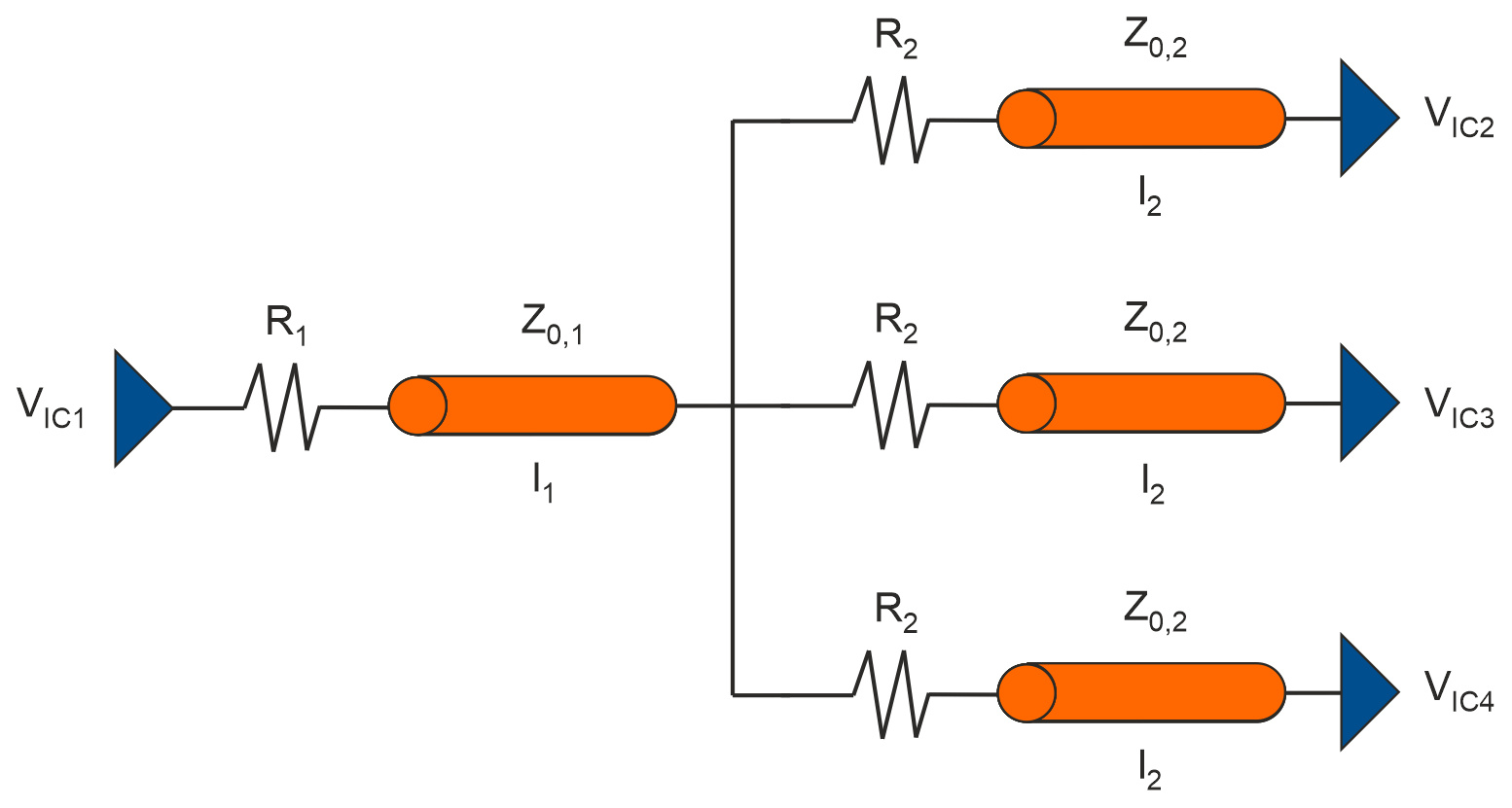
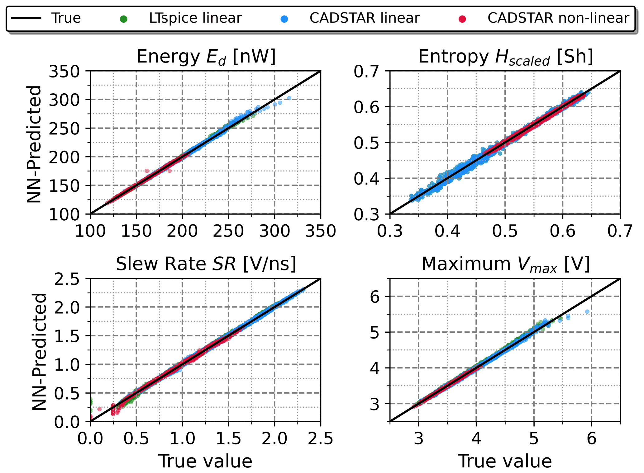
Figure 6 Regression performance of the forward NN model with the BO hyperparameter configuration in terms of true vs. predicted feature values on the entire dataset.

Table 4 R²-Score and RMSE performance metrics of the forward NN with default and BO hyperparameters based on the entire data. Note that additionally the testing metrics are denoted in brackets.

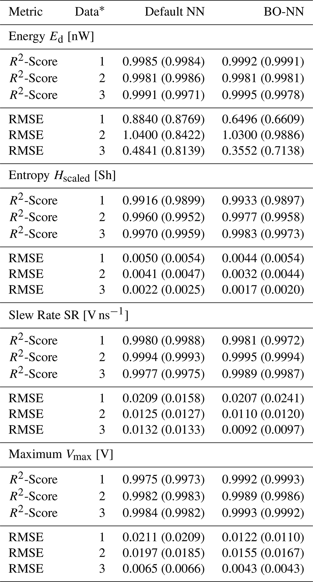
^∗ 1: LTspice linear, 2: CADSTAR linear, 3: CADSTAR non-linear.

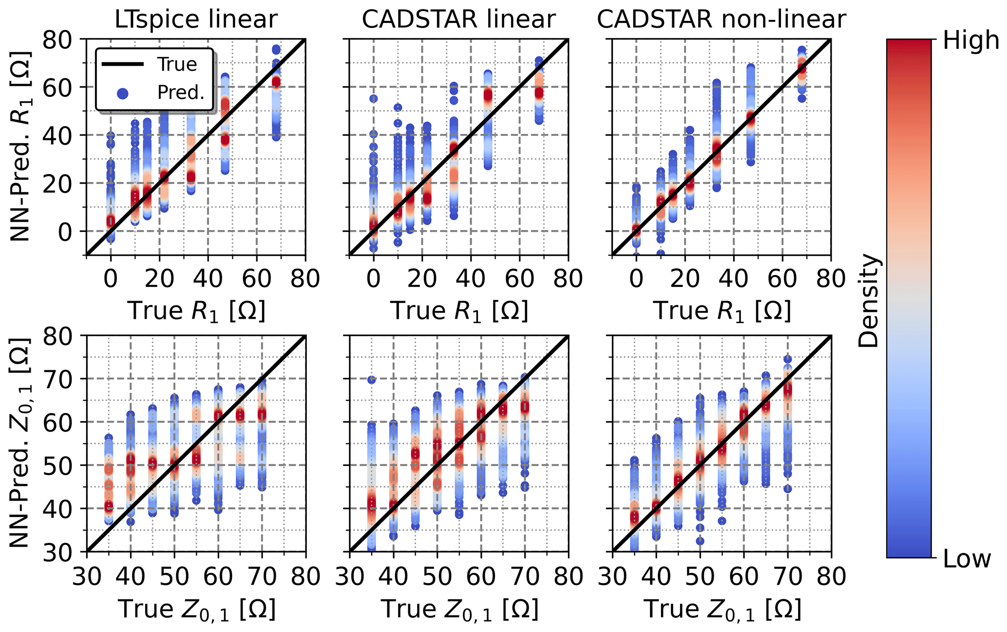
Figure 7 Regression performance of the inverse NN model with the BO hyperparameter configuration in terms of true vs. predicted electrical parameter values exemplary for the prediction of R₁ and Z_0,1. Note that the color-coded density corresponds to the normalized probability density function for each sweeped parameter value.

Table 5 R²-Score and RMSE performance metrics of the inverse NN with default and BO hyperparameters based on the entire data. Note that additionally the testing metrics are denoted in brackets.

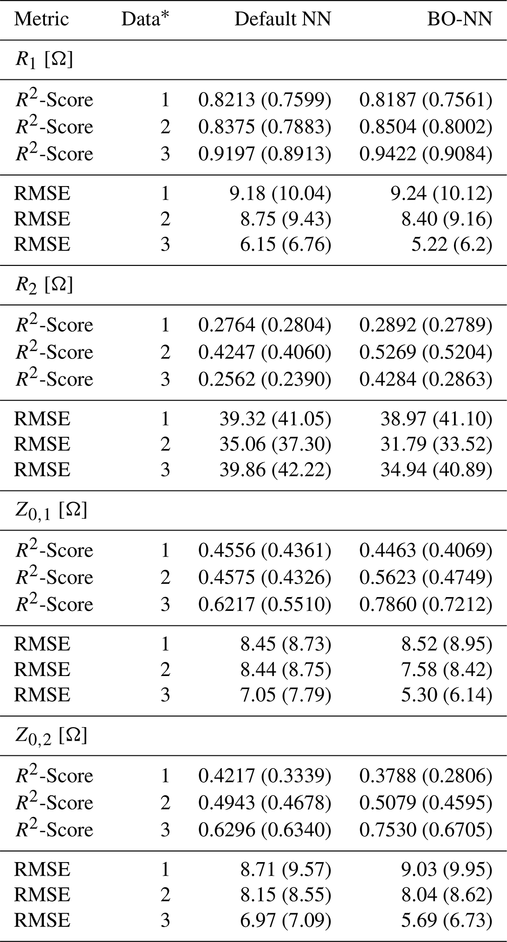
^∗: LTspice linear, 2: CADSTAR linear, 3: CADSTAR non-linear.

Table 6 Feature settings for three defined cases and considered simulation data sources.

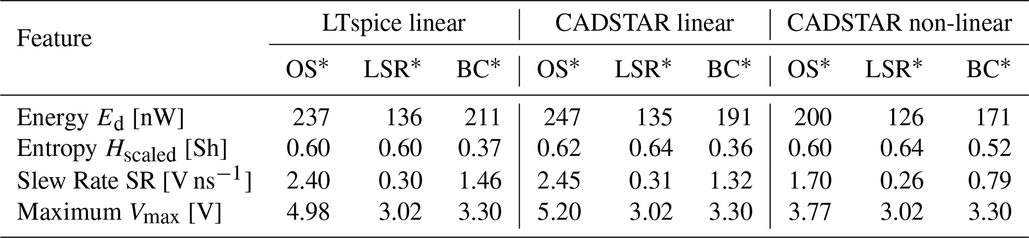
^∗ OS: Worst Case – Overshoot; LSR: Worst Case – Low Slew Rate; BC: Best Case.

Second, the inverse NN regression has been examined, whose regression performance on the entire dataset is exemplary demonstrated for the prediction of R₁ and Z_0,1 in Fig. 7. As expected, the regression performance was evidently impaired by the ambiguity of the non-injective learning function, whose mapping consists of multiple sets of electrical parameters corresponding to matching feature settings. However, the color-coded probability density indicates that a larger proportion of predictions is more accurate, while the deviating cases are statistically more unlikely. Furthermore, the regression performance depends on the relative influence of each electrical parameter with respect to the features. This observation is evident from the testing metric results shown in Table 5 with testing R²-Scores ranging from 24 % to 90 % and testing RMSEs in the range between 6 to 42 Ω with R₁ being predicted with the highest and R₂ with the lowest accuracy. The regression performance of the NN based on the non-linear data has been substantially higher than for the NN models trained with the linear data. This result can be explained by the more realistic modeling of the IC characteristics in the non-linear case. The BO-based hyperparameter tuning affects the NN trained with non-linear data and reduces the RMSE effectively, while at the same time this effect cannot be observed for the NNs trained with linear data. However, the stated higher regression performance of the NN based on the non-linear data is visible for both, the BO and default hyperparameter configurations.

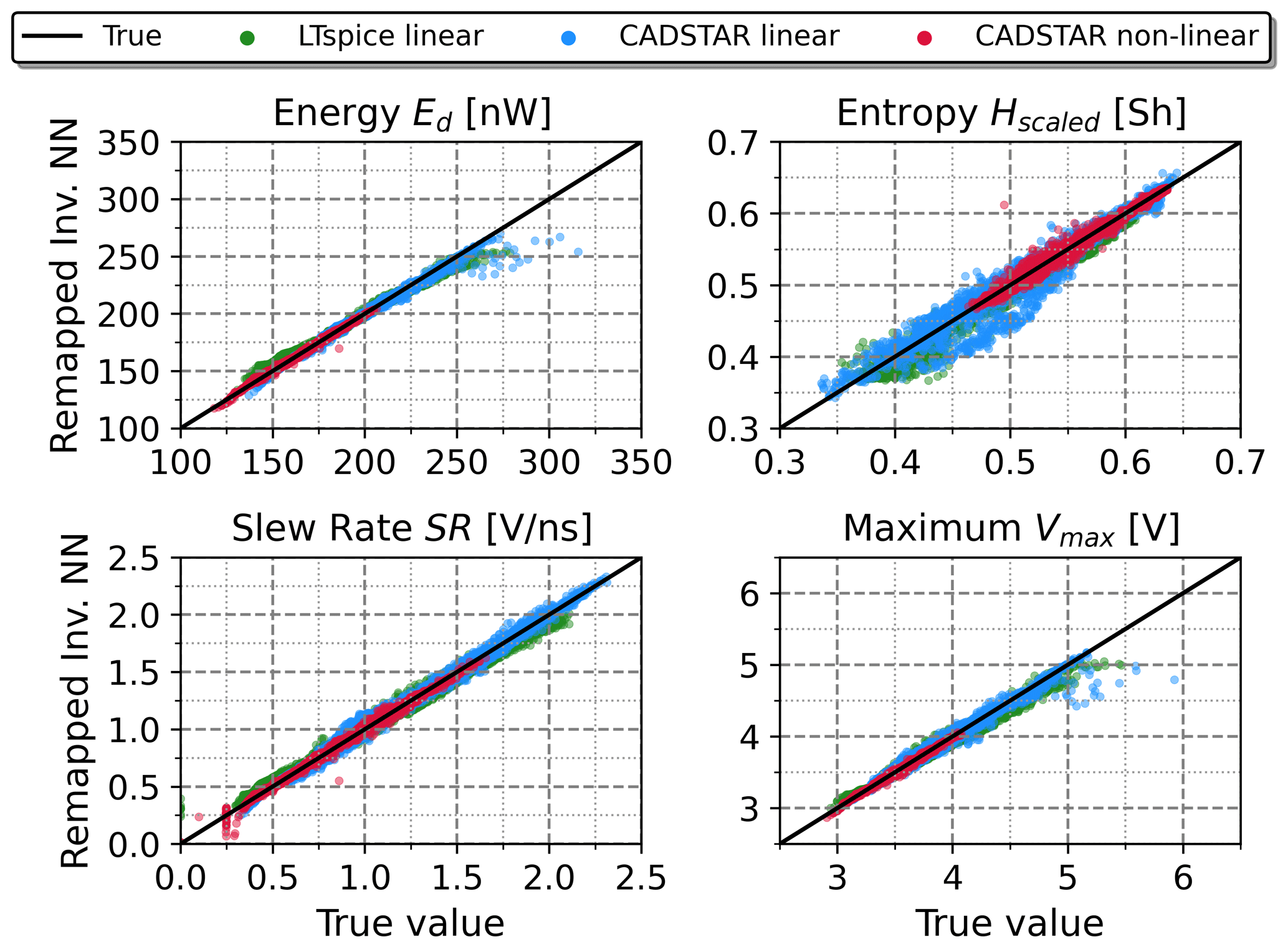
Figure 8 Comparison between the features obtained using the remapping approach based on the inverse NN model and the true feature values.

A second verification of the inverse NN regression has been performed using a forward remapping as shown in Fig. 8. The inverse predicted electrical parameters, which had been determined based on features resulting from simulation data, have been re-mapped into the feature space once again utilizing the previously trained forward NN model, see Fig. 6. The utilization of the forward model instead of resimulations has been chosen to prevent long simulation runs required for the large number of examples. Moreover, the forward NN model has proven to be very accurate in predicting the features, while also offering direct comparability of the re-mapped results with the stand-alone forward model. When comparing the remapping of Fig. 8 with the forward model of Fig. 6, a degradation in performance is evident, which can be traced back to the error induced by the inverse NN model. This is also supported by the quality metrics as the R²-Scores drop by a few percent and the RMSE values at least double throughout the observations. However, the induced error seems to be acceptable especially compared with the direct inverse NN results obtained in Fig. 7 and under the aspect that the forward model achieved a very high accuracy. The second verification of the inverse NN regression therefore provides a first assessment on how much the prediction error of the electrical parameters will affect the features and therefore also the predicted signal behavior.

Table 7 Electrical parameters predicted by the inverse NN based on the feature settings of Table 6.

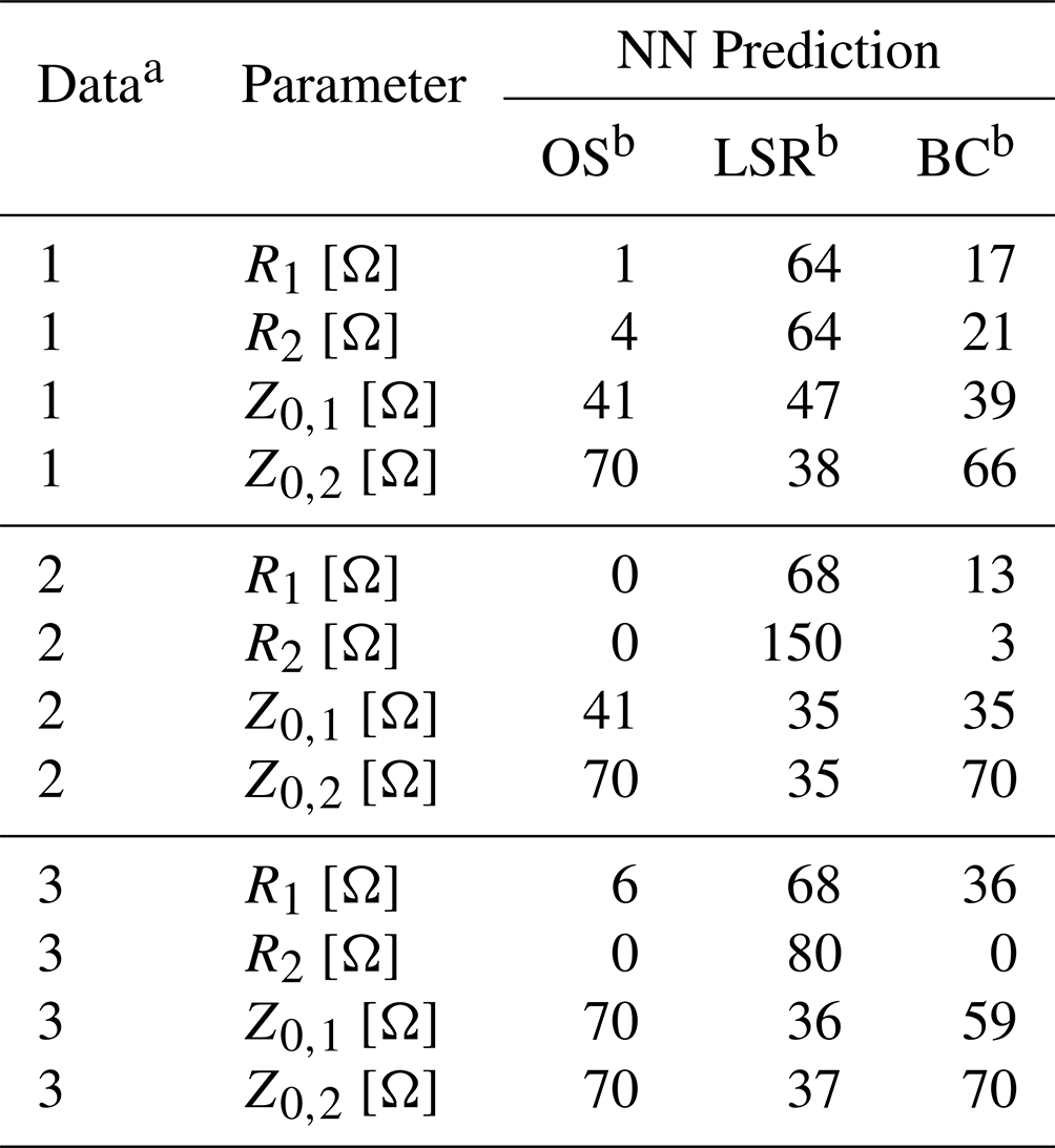
^a: LTspice linear, 2: CADSTAR linear, 3: CADSTAR non-linear. ^b OS: Worst Case - Overshoot, LSR: Worst Case – Low Slew Rate, BC: Best Case.

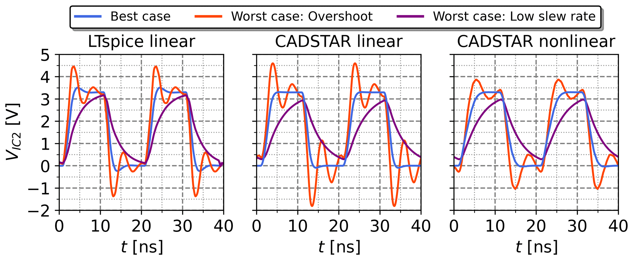
Figure 9 Voltage waveforms resulting from the electrical parameters predicted by the inverse NN based on the feature settings of Table 6.

Based on the feature settings of Table 6, the inverse NN model has been tested using real application cases by analyzing the voltage waveforms resulting from the predicted electrical parameters shown in Table 7. These voltage waveforms are visualized for each of the three cases and for each of the three considered simulation datasets in Fig. 9. These show a distinctive behavior for each case, while also matching the expected signal shape. This confirms the suitability of the inverse NN model within a typical use case. Minor overshoots can be observed for the best case of the models trained with the linear datasets, which is most certainly caused by the inferior regression performance in comparison to the model trained with the non-linear dataset.

5.2 k-Nearest Neighbor

The kNN algorithm has been applied for a feature-based pre-selection based on the cases of Table 6 and was then coupled with the prediction of the inverse NN. The resulting voltage waveforms for each of the cases and simulation datasets are demonstrated in Fig. 10. The voltage waveforms show a distinctive behavior matching the expectations for each case and a very similar behavior for each of the k signals per case. Only small deviations for the best case of linear datasets are observable, which is in accordance with the stand-alone application of the inverse NN in Fig. 9. In general, the voltage waveforms confirm the quality of the proposed combined kNN-NN approach.

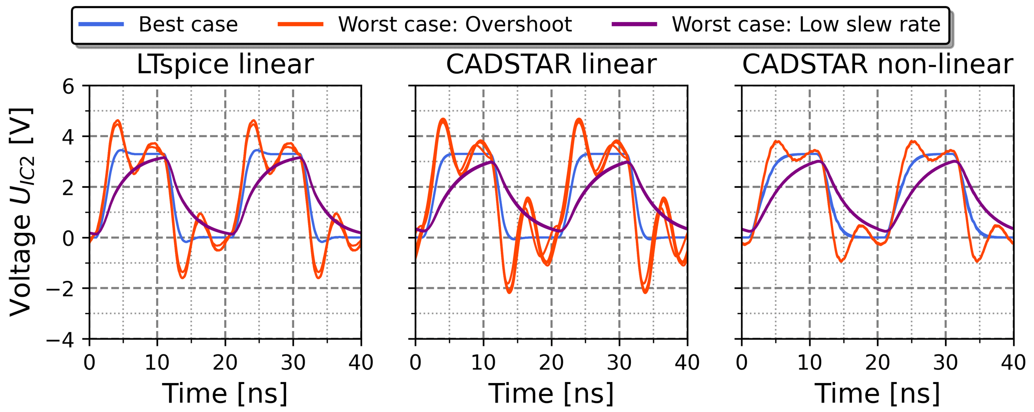
Figure 10 k=5 voltage waveforms resulting from the application of the kNN-NN combination based on the feature settings of Table 6.

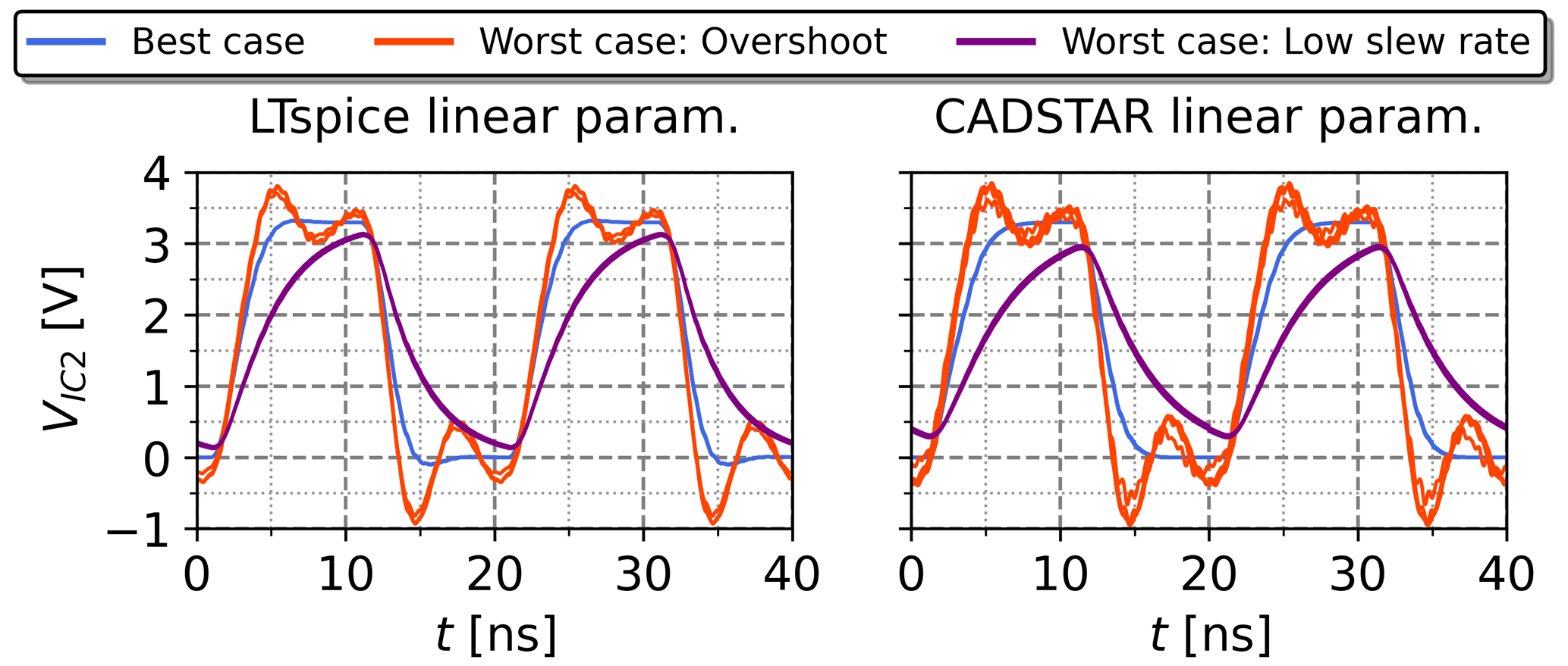
Figure 11 k=5 voltage waveforms simulated with non-linear IBIS models, but parameterized with the kNN-NN combination based on the linear datasets and the feature settings of Table 6.

To further evaluate the portability between the linear and non-linear data using the proposed kNN-NN method, the direct application has been taken into consideration. Therefore, the electrical parameters resulting from the kNN-NN approach, which were entirely determined based on the linear data, have been extracted and resimulated with non-linear IC characteristics. The result is shown in Fig. 11 and demonstrates how the kNN-NN approach deployed with linear data can be directly applied to perform accurate SI analysis with respect to non-linear IC characteristics for the investigated topology.

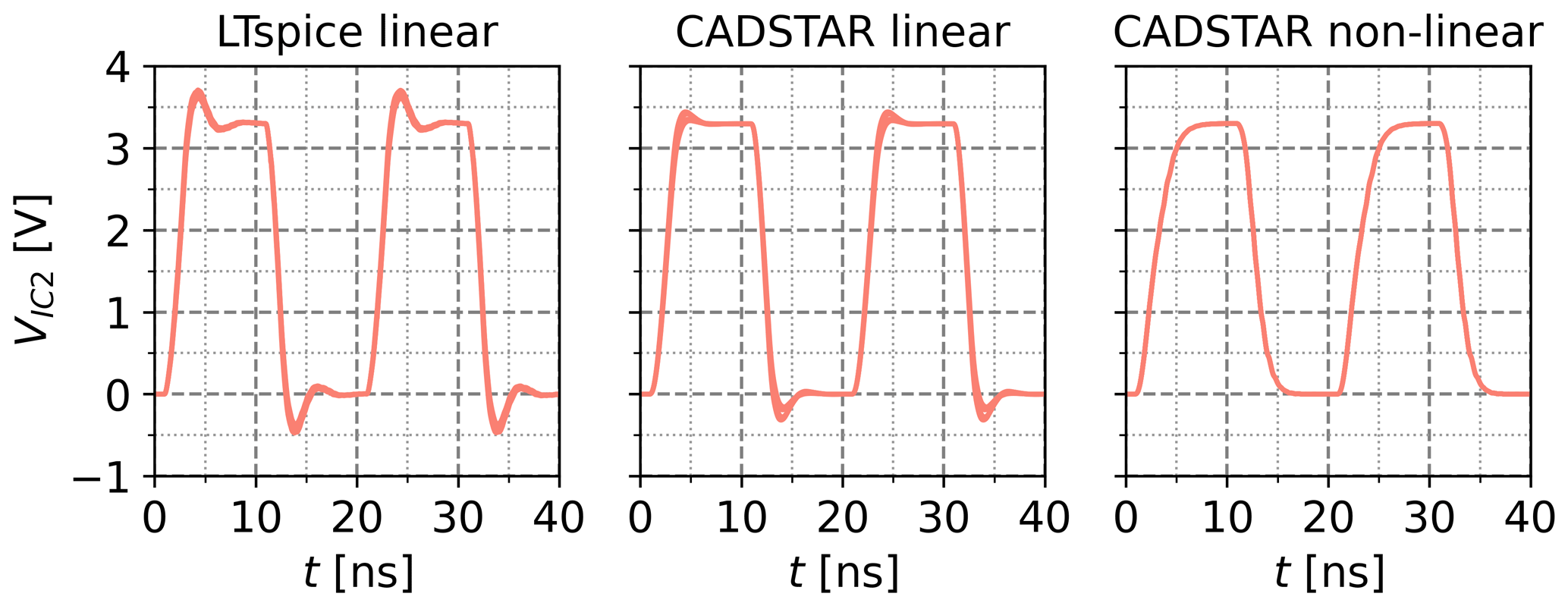
Figure 12 k=5 voltage waveforms resulting from the application of the kNN-NN combination with a feature setting analogical to O₂.

In alternative investigations, the kNN algorithm has been initialized similarly to the GA optimization objective defined in Eq. (10) by setting the energy and slew rate features to the maximum and entropy and maximum voltage features to the minimum normalized value i.e. one and zero, respectively. The resulting voltage waveforms of this kNN initialization with subsequent inverse NN coupling are shown for each of the simulation datasets in Fig. 12. The practical applicability of this approach is proven as the parameterized designs generally exhibit SI-aware behavior. Only for the linear data sources some overshoot behavior is visible, which is consistent with previous results.

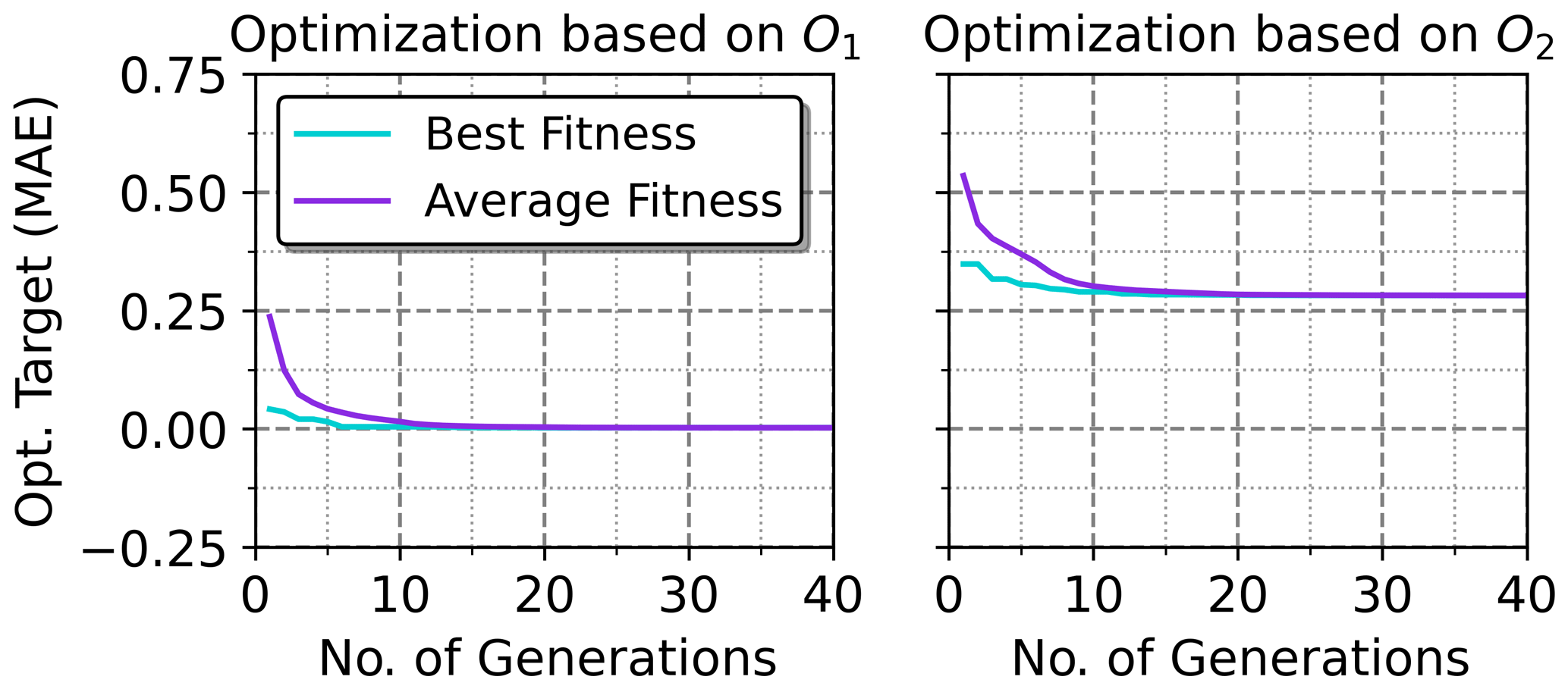
Figure 13 Convergence of the GA over its generations with average and best fitness MAE objective values shown for the CADSTAR linear dataset. Similar convergence behavior has been observed for the other two datasets also.

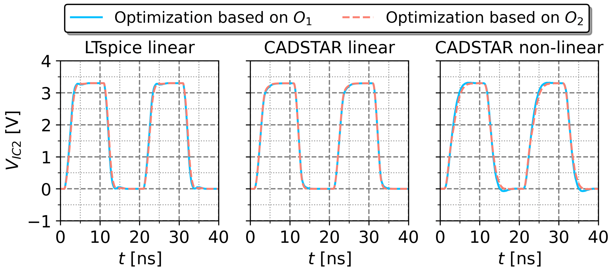
Figure 14 Voltage waveforms resulting from the electrical parameters optimized by the GA based on the objectives O₁ and O₂.

Table 8 Electrical parameters optimized by the GA based on objective O₁ and objective O₂.

^∗: LTspice linear, 2: CADSTAR linear, 3: CADSTAR non-linear.

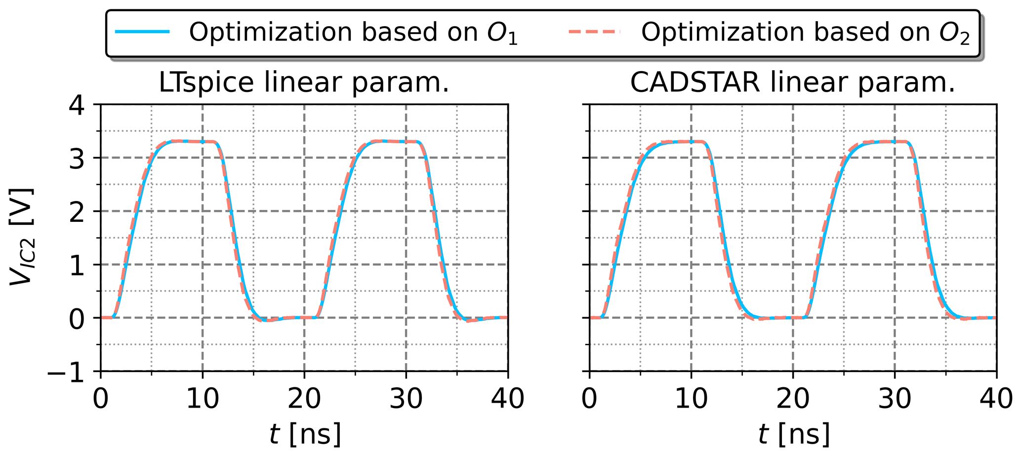
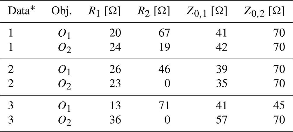
Figure 15 Voltage waveforms simulated with non-linear IBIS models, but parameterized by the GA optimization based on the objectives O₁ and O₂.

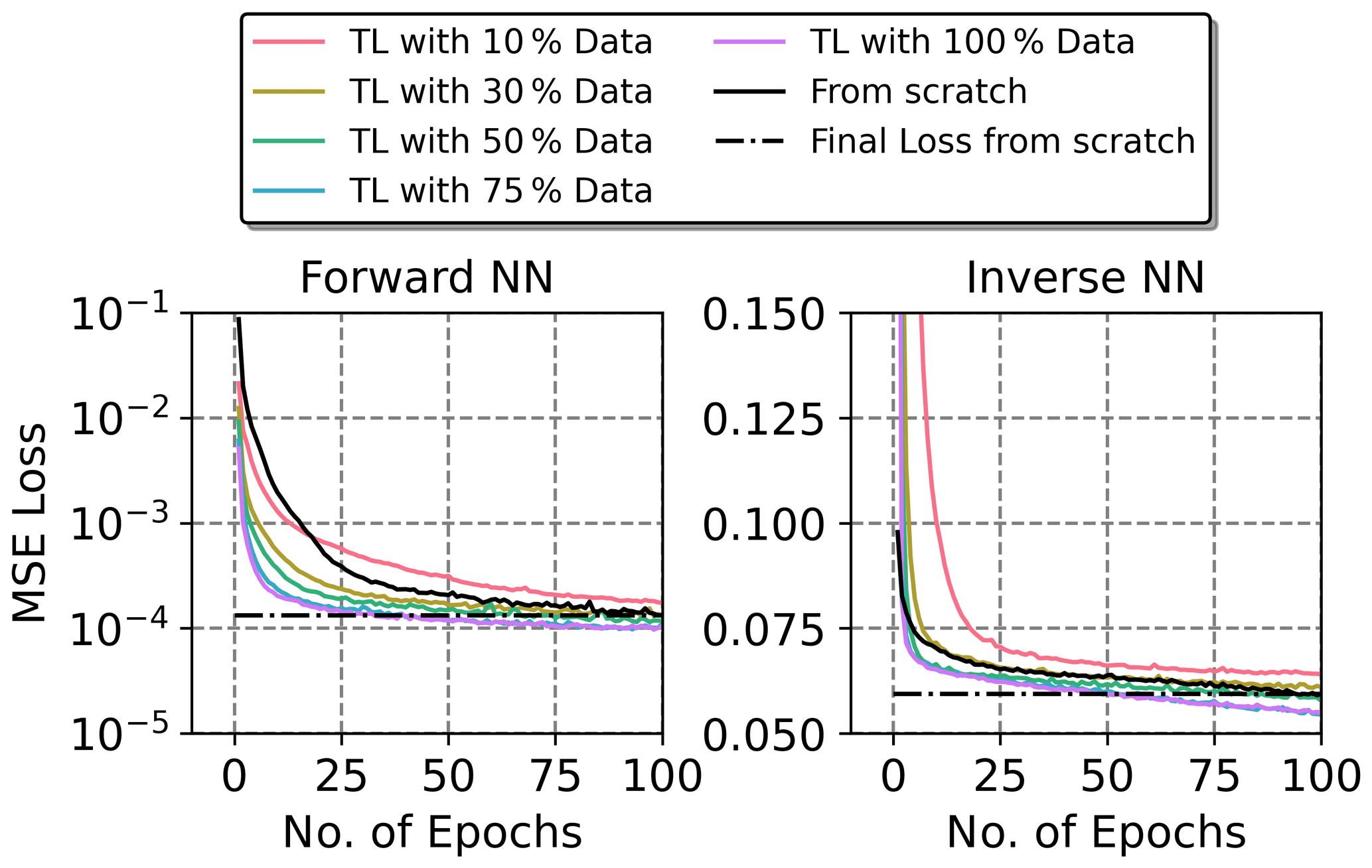
Figure 16 MSE training loss over epochs development during the transfer learning process with different data fractions compared to the training with non-linear data from scratch. Note the logarithmic scaling of the y-axis in case of the forward NN.

5.3 Genetic Algorithms

The GA has been applied to select the optimal electrical parameters within the feature space based on the forward NN model using the two optimization objectives defined in the Eqs. (9) and (10) with F_target equivalent to the best case feature settings of Table 6. For both objectives, the duration of the GA was below 30 s on a common hardware setup. The convergence history of the algorithms is shown for the CADSTAR linear dataset in Fig. 13. It is visible that convergence to a minimum value sets in for both objectives. As expected, the final MAE converges to zero for the first objective, which implies that the distance to the defined best case feature setting embedded into the design space is effectively minimized. For the second objective, a larger residual error remains as the objective can only partly be fulfilled. Due to the physical background of the optimization problem, the possible solution space is limited to valid parameters within the design space. The concurrent optimization of objective O₂ forbids that each feature can be completely maximized or minimized, as this would lead to non-physical solutions, which are intrinsically not allowed. Therefore, the residual MAE indicating the average absolute deviation from the desired target remains above 25 %. The voltage waveforms resulting from the optimized electrical parameters demonstrated in Table 8 are shown in Fig. 14. SI-aware designs have been observed throughout the objectives as well as the different data sources, which validates the usability of the proposed GA method for design optimization tasks.

The direct portability between linear and non-linear data has been evaluated for the utilization of the GA method also. Therefore, the electrical parameters resulting from the GA optimization based on linear data, see Table 8, were extracted and resimulated with non-linear IC characteristics. The resulting voltage waveforms are shown in Fig. 11 and validate that the GA based on linear data can be directly applied to provide accurate SI analysis with respect to non-linear IC characteristics for the investigated topology.

5.4 Transfer Learning

The transfer learning concept, which is also known as fine-tuning, offers another option to ensure portability between the NN architectures trained with linear and non-linear data. The implemented transfer learning has been applied based on a NN pre-trained with the CADSTAR linear dataset, which was then fine-tuned with 100 epochs of the non-linear data. Moreover, the transfer learning applications were applied with various fractions of data such as 10 %, 30 %, 50 %, 75 % and 100 %, which have been randomly sampled from the original dataset. Figure 16 shows the MSE loss over epochs development of the transfer learning process for the forward and inverse mode regression. It is apparent that with data fractions of 50 % and above, the convergence was accelerated resulting in a lower loss after 100 epochs for both, the forward and inverse mode regression, compared to the training from scratch. This is due to the learned knowledge representations contained in the pre-trained NNs. Compared to the training from scratch with a data fraction of 30 %, the training MSE loss of the forward transfer learning was at least on a par and the inverse transfer learning was slightly impaired. Finally, for the transfer learning with a fraction of 10 % the amount of data apparently falls below the threshold of required data quantity as the MSE training loss was significantly higher compared to the from scratch trained model for both, the forward and inverse transfer learning. Overall, the application of transfer learning between linear and non-linear IC characteristics entails significant simplifications of the data generation and training processes. The fine-tuning on an existing model that has been trained based on linear data enables savings of at least 50 % during the data generation with non-linear IC characteristics, which then also effectively reduces training complexity and computation times.

6 Conclusions and Future Work

The two-stage AI framework presented in this paper has been validated to support the application in the PCB design process with respect to linear and non-linear data. SI-compliant designs were obtained using the forward NN in combination with a GA for optimization as well as the inverse NN in combination with the kNN algorithm. The different data sources only affected the performance with respect to the inverse NN as the regression accuracy was significantly improved when utilizing the non-linear data. In this context, the NN hyperparameter tuning with BO also had a significant impact in further improving the regression performance, which is in contrast to the other results, where the impact of hyperparameter tuning with BO was marginal at best. Furthermore, it has also been shown that for the investigated application the designs parameterized using the AI framework based on linear datasets can be successfully applied to provide SI design support valid for the non-linear IC characteristics also. Alternatively, the transfer learning capabilities of the NNs have been evaluated for fine-tuning of the models trained with linear data using different fractions of non-linear data. These investigations showed that at least 50 % of the training data can be saved to achieve the same or even improved regression performance.

Future research may incorporate the application of the presented AI framework to technologies from the DDR-SDRAM class such as DDR3/4/5 with much shorter rise- and fall times operating at higher clock frequencies and lower voltage levels to investigate the portability and adaptability of the developed AI models. In particular, the transfer of the developed AI models for different component technologies into practice-oriented AI modules (deployment) will be an important subject. In this context, the further integration of SI constraints will be of great importance, especially considering the timing and resulting skew characteristics of the signals, which also requires a more differentiated examination of the feature selection. Furthermore, the constraint integration during the parameterization stage may include feature weighting and multi-objective optimization methods to provide customization to the developer's needs. In the end, combining the forward and inverse NN models in the first AI stage as well as different parameterization methods such as kNN and GA in the second AI stage within an iterative process may yield synergy effects resulting in significant improvements of the framework.