Comparison of Inductive and Capacitive End Couplings in the Design of a Combline Microwave Cavity Filter for the E1 Galileo Band

Inductive and capacitive end couplings in the design of combline microwave filters are compared. For instance, a combline microwave cavity filter for the E1 Galileo band (1559–1591 MHz, 2 % fractional bandwidth) is considered. The inductive end coupling is composed of an L-shaped pin in galvanic contact with the end resonator, while the capacitive end coupling is realized by a straight pin parallel to the end resonator's axis. Although both end couplings can realize the desired external quality factor, the capacitive end coupling is easier to manufacture, while the inductive end coupling is less sensitive to the design parameter. An excellent agreement between synthesized (5th-order Chebyshev mask with 0.05 dB ripple) and measured responses is observed for the realized prototype of the filter. The insertion losses at the center frequency are 1.72 and 1.53 dB for the inductive and capacitive end couplings, respectively. The spurious-free ranges are up to 8.23 and 8.92 GHz for inductive and capacitive end couplings, respectively.

1 Introduction

Microwave cavity filters are commonly used in many applications, e.g., in low-level RF systems (Piersanti et al., 2021, 2023) and in satellite communications (Judith Sen et al., 2017; Zhang et al., 2021). Microwave cavity filters are used in these fields due to their high selectivity which allows one to reject signals close in frequency. Despite being widely analyzed in the 1970s and in the 1980s (Wenzel, 1971; Matthaei et al., 1980), combline filters are still of interest nowadays (Xu et al., 2019; Vague et al., 2021; Jamshidi-Zarmehri et al., 2023).

A feature of microwave filters is the end coupling (Swanson, 2007), which is important in achieving the desired filter response and can be realized with different schemes. For example, the coaxial cable can enter the cavity right-angle (Rudakov et al., 2013) or in-line (Gatti et al., 2019). The coupling can require contact if inductive (Cristal, 1975; Anwar and Dhanyal, 2018) or not if capacitive (Judith Sen et al., 2017; Chu and Zhang, 2017). The capacitive coupling is gaining interest, as it is easier to manufacture (Gatti et al., 2019) than the inductive coupling and is applicable to tunable filters requiring a mobile post (Widaa et al., 2023).

Here two different end couplings are compared. They are of inductive and capacitive types, and they are investigated numerically in Boni et al. (2023c, a), respectively. Then, the present work extends the numerical results there presented by providing measured results for both kinds of end couplings. To the best of our knowledge, this is the first time such a comparison has been carried out.

As a practical instance, the comparison is performed considering an L-band combline microwave filter that receives the E1 Galileo signal (1559–1591 MHz) (Hegarty, 2012) and rejects the Iridium signal (1616–1626.5 MHz) (Pratt et al., 2009). In particular, the filter is needed to equip LaBarchettaMagica of the project VELA (Boni et al., 2023b, 2020), a demonstrator of an autonomous ship.

The article is organized as follows. In Sect. 2, the specifications and the respective coupling matrix for the filter serving as an example are provided and the combline microwave cavity filter is designed, focusing on the end coupling. Then, in Sect. 3 the measured results are presented. Finally, the conclusion is drawn in Sect. 4.

2 Filter design

2.1 Specifications

The bandwidth of the E1 Galileo signal is f₁=1559–f₂=1591 MHz. The center frequency is $f_{\mathrm{0}}=\sqrt{f_{\mathrm{1}}{f}_{\mathrm{2}}}=\mathrm{1575}$ MHz, the bandwidth $\text{BW}=f_{\mathrm{2}}-f_{\mathrm{1}}=\mathrm{32}$ MHz, and the fractional bandwidth $\text{FBW}=\text{BW}/f_{\mathrm{0}}=\mathrm{2}$ % (Boni et al., 2022). A Chebyshev mask is chosen for its steeper roll-off at the passband edges, when compared to the Butterworth mask. Then, to have an insertion loss greater than 40 dB in the Iridium band (1616–1626.5 MHz), a filter order of at least N=5 is needed. To achieve a good matching in the passband, a ripple of 0.05 dB (minimum return loss in passband equal to 19.41 dB) for the synthesized Chebyshev response is considered.

2.2 Coupling matrix

For the given synthesized response, the coupling matrix M=M^T has dimension $(N+\mathrm{2})\times (N+\mathrm{2})$ and its expression is

$$\begin{array}{}\text{(1)}& \mathbf{M}=\left(\begin{array}{ccccccc}\mathrm{0}& m_{\mathrm{0},\mathrm{1}}& \mathrm{0}& \mathrm{0}& \mathrm{0}& \mathrm{0}& \mathrm{0}\\ m_{\mathrm{1},\mathrm{0}}& \mathrm{0}& m_{\mathrm{1},\mathrm{2}}& \mathrm{0}& \mathrm{0}& \mathrm{0}& \mathrm{0}\\ \mathrm{0}& m_{\mathrm{2},\mathrm{1}}& \mathrm{0}& m_{\mathrm{2},\mathrm{3}}& \mathrm{0}& \mathrm{0}& \mathrm{0}\\ \mathrm{0}& \mathrm{0}& m_{\mathrm{3},\mathrm{2}}& \mathrm{0}& m_{\mathrm{3},\mathrm{4}}& \mathrm{0}& \mathrm{0}\\ \mathrm{0}& \mathrm{0}& \mathrm{0}& m_{\mathrm{4},\mathrm{3}}& \mathrm{0}& m_{\mathrm{4},\mathrm{5}}& \mathrm{0}\\ \mathrm{0}& \mathrm{0}& \mathrm{0}& \mathrm{0}& m_{\mathrm{5},\mathrm{4}}& \mathrm{0}& m_{\mathrm{5},\mathrm{6}}\\ \mathrm{0}& \mathrm{0}& \mathrm{0}& \mathrm{0}& \mathrm{0}& m_{\mathrm{6},\mathrm{5}}& \mathrm{0}\end{array}\right)\end{array}$$

where $m_{i,i+\mathrm{1}}$ is the normalized coupling coefficient between resonators i and i+1 and it is given by

$$\begin{array}{}\text{(2)}& m_{i,i+\mathrm{1}}={\displaystyle \frac{\mathrm{1}}{\sqrt{g_i{g}_{i+\mathrm{1}}}}},i=\mathrm{0},\mathrm{1},\mathrm{2},\mathrm{\dots },N-\mathrm{1},N,\end{array}$$

being g_i the ith immitance of the low pass prototype. For the given Chebyshev prototype response, the immittances of the low-pass prototype are $g_{\mathrm{0}}=g_{\mathrm{6}}=\mathrm{1}$, $g_{\mathrm{1}}=g_{\mathrm{5}}=\mathrm{0.9984}$, $g_{\mathrm{2}}=g_{\mathrm{4}}=\mathrm{1.3745}$, g₃=1.8283. Then, the numerical values of the normalized coupling coefficients are

$$\begin{array}{}\text{(3a)}& {\displaystyle }{m}_{\mathrm{1},\mathrm{0}}=m_{\mathrm{0},\mathrm{1}}=m_{\mathrm{5},\mathrm{6}}=m_{\mathrm{6},\mathrm{5}}=\mathrm{1.001}\text{(3b)}& {\displaystyle }{m}_{\mathrm{1},\mathrm{2}}=m_{\mathrm{2},\mathrm{1}}=m_{\mathrm{4},\mathrm{5}}=m_{\mathrm{5},\mathrm{4}}=\mathrm{0.854}\text{(3c)}& {\displaystyle }{m}_{\mathrm{2},\mathrm{3}}=m_{\mathrm{3},\mathrm{2}}=m_{\mathrm{3},\mathrm{4}}=m_{\mathrm{4},\mathrm{3}}=\mathrm{0.631}.\end{array}$$

The external quality factor of input and output ports is instead given by

$$\begin{array}{}\text{(4)}& Q_{\mathrm{E}}={\displaystyle \frac{\mathrm{1}}{m_{\mathrm{0},\mathrm{1}}^{\mathrm{2}}\text{FBW}}}={\displaystyle \frac{\mathrm{1}}{m_{\mathrm{5},\mathrm{6}}^{\mathrm{2}}\text{FBW}}}\end{array}$$

and it turns out that Q_E=49.1. For completeness, the coupling bandwidths CBWs are computed as

$$\begin{array}{}\text{(5)}& {\text{CBW}}_{i,i+\mathrm{1}}=m_{i,i+\mathrm{1}}\cdot \text{BW},i=\mathrm{0},\mathrm{1},\mathrm{2},\mathrm{\dots },N-\mathrm{1},N\end{array}$$

and their values are

$$\begin{array}{}\text{(6a)}& {\displaystyle }{\text{CBW}}_{\mathrm{1},\mathrm{2}}={\text{CBW}}_{\mathrm{4},\mathrm{5}}=\mathrm{27.3}\text{MHz}\text{(6b)}& {\displaystyle }{\text{CBW}}_{\mathrm{2},\mathrm{3}}={\text{CBW}}_{\mathrm{3},\mathrm{4}}=\mathrm{20.2}\text{MHz}.\end{array}$$

2.3 Filter technology and dimensions

There are several ways to obtain a physical description of the filter starting from the coupling matrix. Hereinafter, the combline coaxial filter technology is considered (Anwar and Dhanyal, 2018).

The combline coaxial cavity filter is composed of coaxial resonators (shunt resonators realized using shorted transmission lines and loaded with a capacitance at the other end) of physical length $L={\mathit{\lambda }}_{\mathrm{0}}/\mathrm{8}=\mathrm{23.8}$ mm, with λ₀=190.3 mm the wavelength at f₀ in vacuum. The number of resonators is equal to the filter order.

A rectangular aluminum cavity encloses the resonators. For unavoidable post-manufacturing tuning, coupling and tuning screws (modeled as circular cylinders) are added to the design. Note that the tuning screws operate on the resonance frequencies of the resonators, while the coupling screws operate on the coupling coefficients between the resonators. In particular, the more the tuning (coupling) screws penetrate, the lower the resonance frequencies of the resonators (the greater the couplings between adjacent resonators).

Figure 1a shows a 3D view of the filter modeled in the full-wave simulator CST (Dassault Systèmes, 2023) and Fig. 1b provides the dimensions. These are the same as those described in Boni et al. (2023c) and the reader is therefore referred to that reference for further details.

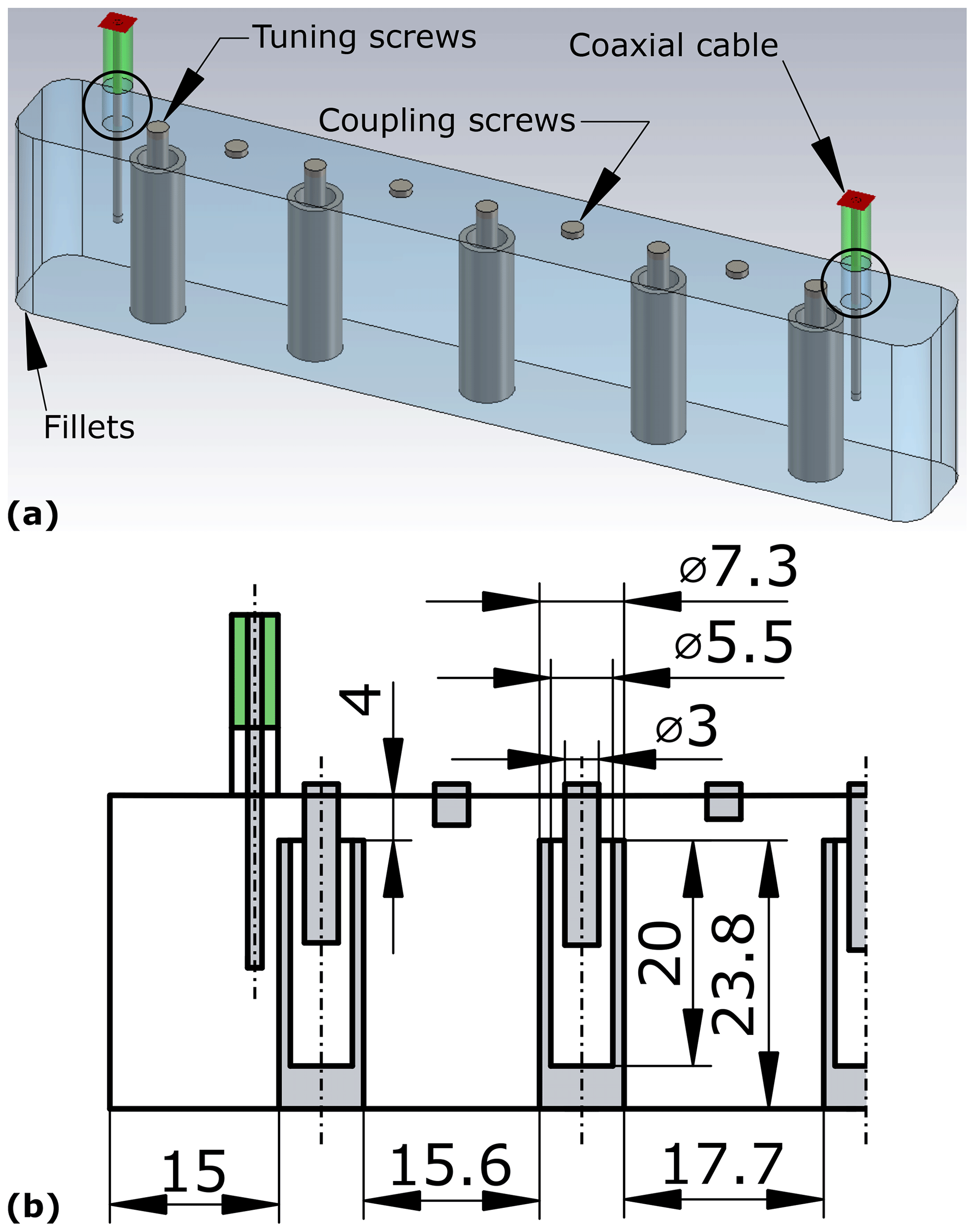
Figure 1 Design of the filter: (a) 3D model simulated in CST; (b) technical drawing with dimensions in millimeters. In panel (a), the extensions inside the circles account for the thickness of the cavity. In panel (b), only one half filter is depicted thanks to its symmetry. The cavity width is 16 mm and the fillet radius is 4 mm.

Due to the complex shape of the filter, for analysis it is not straightforward to rely on semianalytical techniques such as mode matching (Gentili et al., 2023), so we prefer to rely on full-wave simulations. Then, the filter is modeled and simulated in CST. This software is preferred over others because it offers a dedicated package, called Filter Designer 3D, for modeling and fine-tuning of microwave filters. In both simulations and measurements, the filter has been fine-tuned by comparing the realized coupling matrix, extracted by the Filter Designer 3D tool, with the synthesized coupling matrix Eq. (1). This comparison returns indications on the screws to turn and the direction of the screwing.

2.4 End coupling

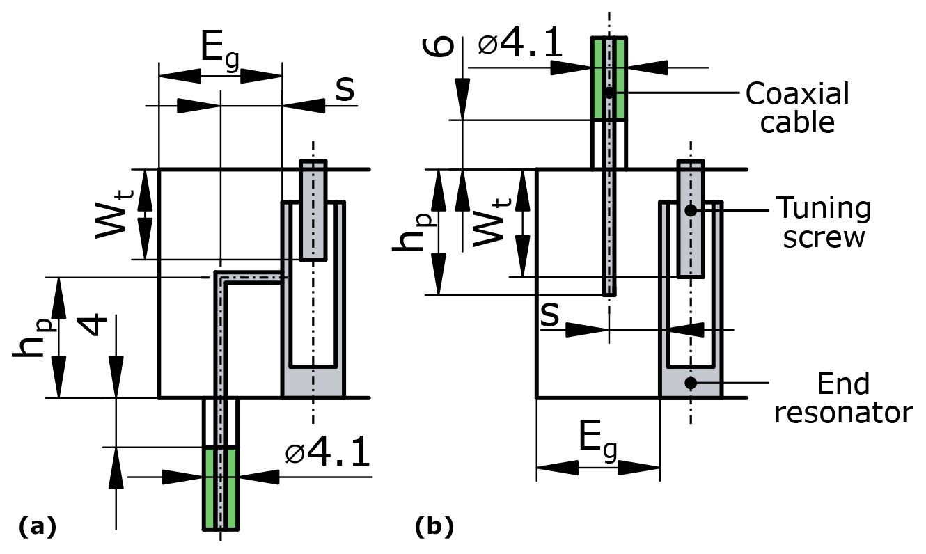
While in Fig. 1 a capacitive end coupling is depicted, both the inductive and capacitive end couplings described in Boni et al. (2023a, c) are realized and compared. Their technical drawings are sketched in Fig. 2. Both end coupling designs are described by three geometric parameters: pin height h_p, distance between the end resonator and the end wall E_g, and distance between the end resonator and the symmetry axis of the connector s. The quantity E_g is kept fixed and equal to 15 mm for both types of end couplings, as drawn in Fig. 1b. The quantity s is equal to $E_{\mathrm{g}}/\mathrm{2}=\mathrm{7.5}$ mm for the inductive end coupling and equal to 3.35 mm for the capacitive end coupling. The pin height h_p is set to achieve the desired value of the external quality factor, as described in Boni et al. (2023a, b, c). The method of finding the pin height is discussed in the following.

Figure 2 Realized end couplings.

3 Results

3.1 Realization

The coaxial resonators are made of brass, while the cavity is made of aluminum (see Fig. 3a). The cavity is divided into two parts, called the main body and the lid (see Fig. 3b). The resonators are fastened to the main body using one M3 screw each, while the lid hosts the threaded holes for the brass tuning and coupling screws. Although bolted joints would be avoided to bypass contact resistance problems (Zhang et al., 2019), the ratio between the height of the cavity and the distance of the resonators from the walls of the cavity is 27.8 to 4.35, thus preventing the use of a standard milling cutter; hence the decision to manufacture the cavity and the resonators separately. The subminiature version A (SMA) connectors are fastened to the main body and the lid for the inductive and capacitive end couplings, respectively. The lid is fastened to the main body using eighteen M2 screws (see Fig. 3c). Two instances of the SMA connectors for inductive and capacitive end couplings are shown in Fig. 3d.

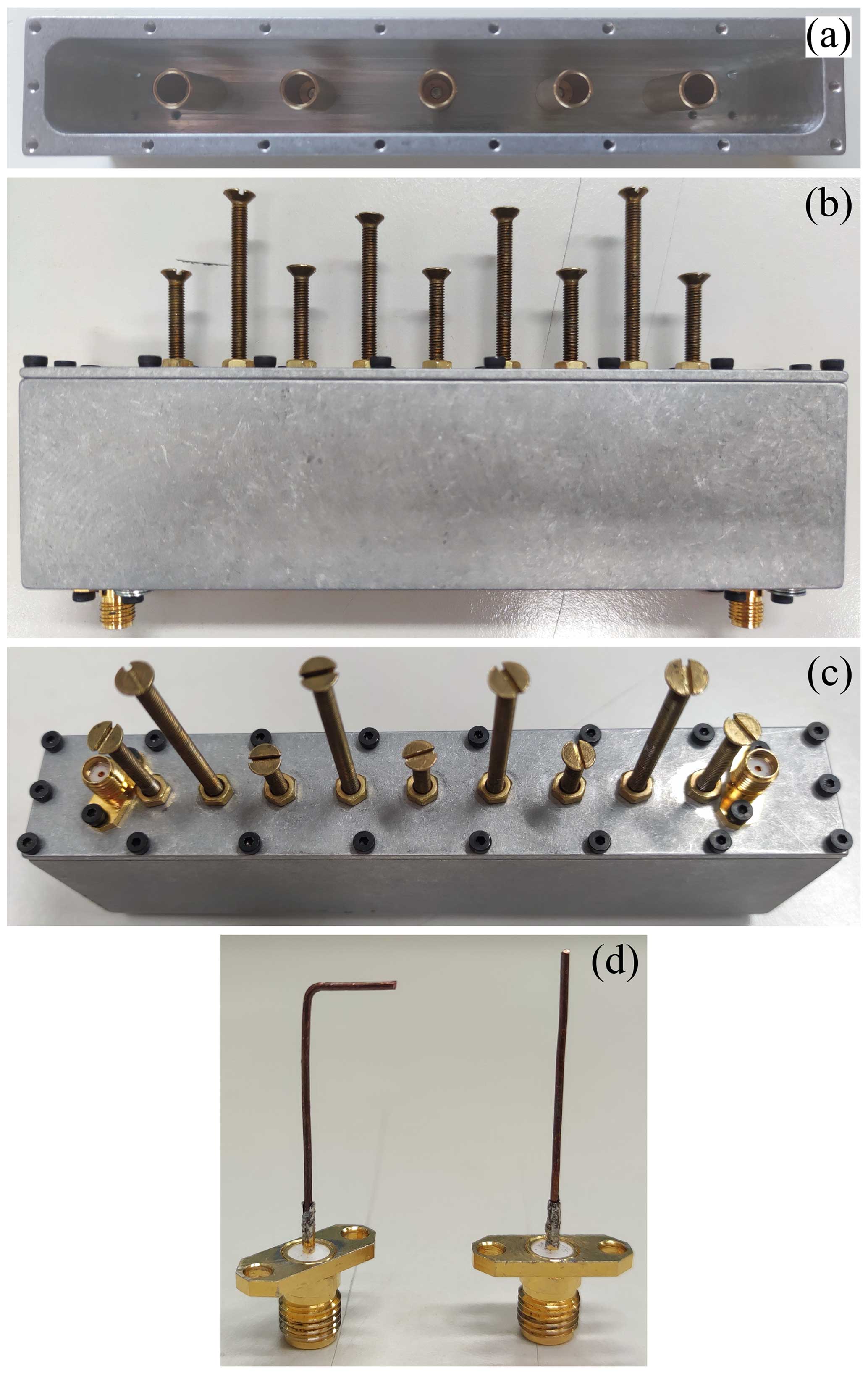
Figure 3 Picture of the manufactured filter: (a) top view without lid (brass resonators are visible); (b) lateral view with inductive end coupling; (c) oblique view with capacitive end coupling; (d) instances of two end couplings: inductive on the left, capacitive on the right.

Both designs of the end coupling allow milling the main body and the lid with a single positioning of the starting aluminum blocks, then having an easier manufacturing process. A single type of end coupling is used at a time. Then, the SMA connector holes for the end coupling not in use are covered with copper tape. Concerning the manufacturing of the filter, the capacitive end coupling has the great advantage that it requires no galvanic contact with the end resonator, thus simplifying the realization. Besides, the capacitive end coupling can be inserted in a closed structure (Gatti et al., 2019).

3.2 Measurements

3.2.1 External quality factor

In the case of over-coupling (Pozar, 2011, pp. 297–300), the external quality factor is related to the group delay Γ_d at the center frequency by (Ness, 1998)

$$\begin{array}{}\text{(7)}& {\displaystyle }{\mathrm{\Gamma }}_{\mathrm{d}}\left(f_{\mathrm{0}}\right)={\displaystyle \frac{\mathrm{2}}{\mathit{\pi }{f}_{\mathrm{0}}}}{\displaystyle \frac{Q_{\mathrm{E}}}{\mathrm{1}-{\left(\frac{Q_{\mathrm{E}}}{Q_{\mathrm{u}}}\right)}^{\mathrm{2}}}}\text{(8)}& {\displaystyle \frac{Q_{\mathrm{E}}}{Q_{\mathrm{u}}}}={\displaystyle \frac{\mathrm{1}-\left|S_{\mathrm{11}}\right(f_{\mathrm{0}}\left)\right|}{\mathrm{1}+\left|S_{\mathrm{11}}\right(f_{\mathrm{0}}\left)\right|}}\end{array}$$

in which Q_u is the unloaded quality factor, and S₁₁(f₀) is the magnitude of the reflection coefficient in linear unit at f₀. Thanks to Eq. (7), the measured external quality factor is corrected to account for the losses. Inverting Eq. (7) and exploiting Eq. (8), it is possible to obtain the external quality factor from the measured group delay. Additionally, the group delay in Eq. (7) is de-embed to account for the extra length of the coaxial cable feeding the filter (Hsu et al., 2002; Boni et al., 2023c).

The external quality factor versus the pin height is shown in Fig. 4. Displayed results are both from measurements and lossy simulations (brass for resonators and screws, copper for the pins, aluminum for the cavity, and loss tangent equal to 0.0002 for the dielectric of the input/output coaxial cables). The simulated data are found by interfacing MATLAB with CST analogously to what is done in Giannetti (2023a). In Fig. 4, the measured point for capacitive coupling and h_p=6 mm is missing since, due to losses, there is under-coupling instead of over-coupling, thus preventing the application of Eqs. (7) and (8). The vertical shift between measured and simulated points is attributable to manufacturing imperfections. These are the misalignment of the SMA connector since its joint with the filter body presents clearance (the SMA connector may be closer to or more distant from the end resonator), the manual production of the end couplings, which may lead to not perfectly straight wires, and the location of the contact point for the inductive coupling, which may change when disassembling and assembling again. For reproducibility, the authors tried to fasten the SMA connector always in the same position, that is, closer to the end resonator. Despite these nonidealities, the trend in the measured external quality factors is well replicated by the trend in the simulated external quality factors.

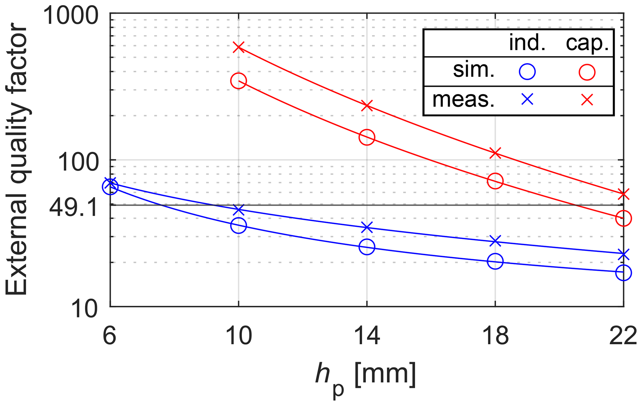
Figure 4 External quality factor versus the pin height. Abbreviations are: sim. for simulations, meas. for measurements, ind. for inductive, and cap. for capacitive. Solid lines indicate the fitting curves.

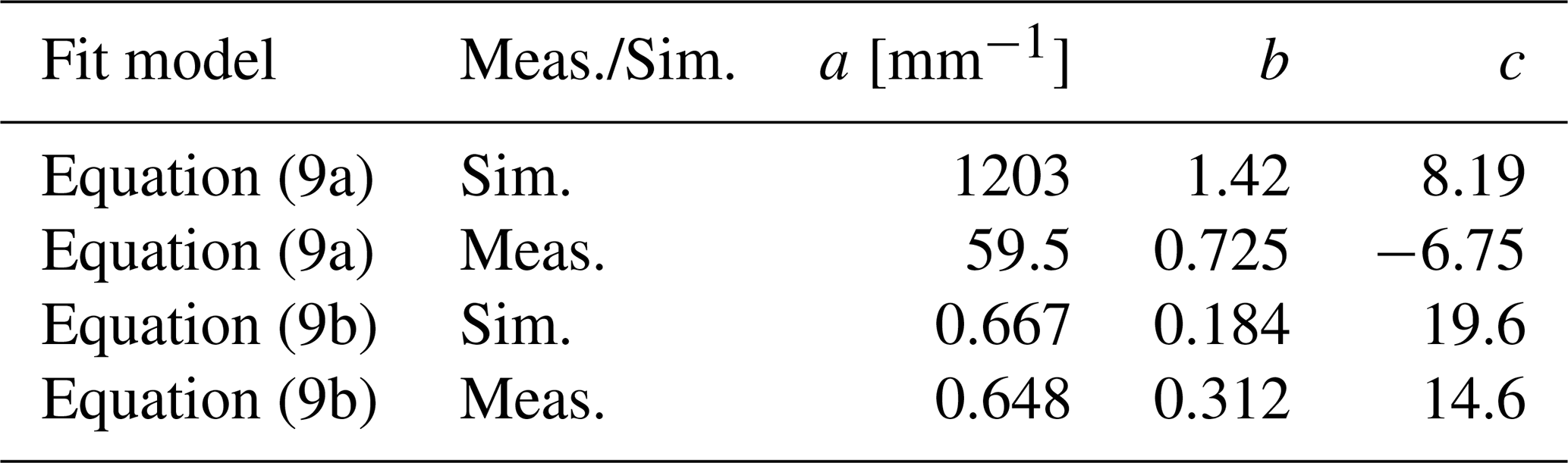
Observing the curves in Fig. 4, the points are fitted with the following heuristic models

$$\begin{array}{}\text{(9a)}& {\displaystyle }{Q}_{\mathrm{E}}& {\displaystyle }=(a{h}_{\mathrm{p}}{)}^{-b}+c& {\displaystyle }\text{inductive coupling}\text{(9b)}& {\displaystyle }{Q}_{\mathrm{E}}& {\displaystyle }=e^{-(a{h}_{\mathrm{p}}{)}^b+c}& {\displaystyle }\text{capacitive coupling}\end{array}$$

where a, b, and c are fitting parameters. These are found to solve a least squares problem and are listed in Table 1 for the four curves. The fitting curves are also drawn in Fig. 4. The capacitive coupling is more sensitive to variations in pin height than the inductive end coupling. This greater sensitivity may be an advantage since it is possible to realize a wider range of external quality factors, but it may be a disadvantage as well since the design is more affected by manufacturing tolerances than the inductive end coupling. After this study, the height of the pin that achieves the desired value of the external quality factor is 9.2 mm (23.2 mm) for the inductive (capacitive) end coupling.

Table 1 Fitting parameters for models Eqs. (9a) and (9b), considering both simulated and measured data.

To qualitatively compare the two end couplings, the maximum phasor amplitude of the current density and the electric field at the center frequency is displayed in Fig. 5. The phasor amplitude of the current density for the inductive end coupling is homogeneous all along the pin, while it assumes low values on the side of the pin facing the end resonator for the capacitive end coupling. The phasor amplitude of the current density for the end resonator is similar for the two end couplings. The maximum phasor amplitude for the electric field is stronger for the capacitive end coupling than for the inductive end coupling, as expected. In particular, it is more intense on the part of the capacitive probe facing the end resonator.

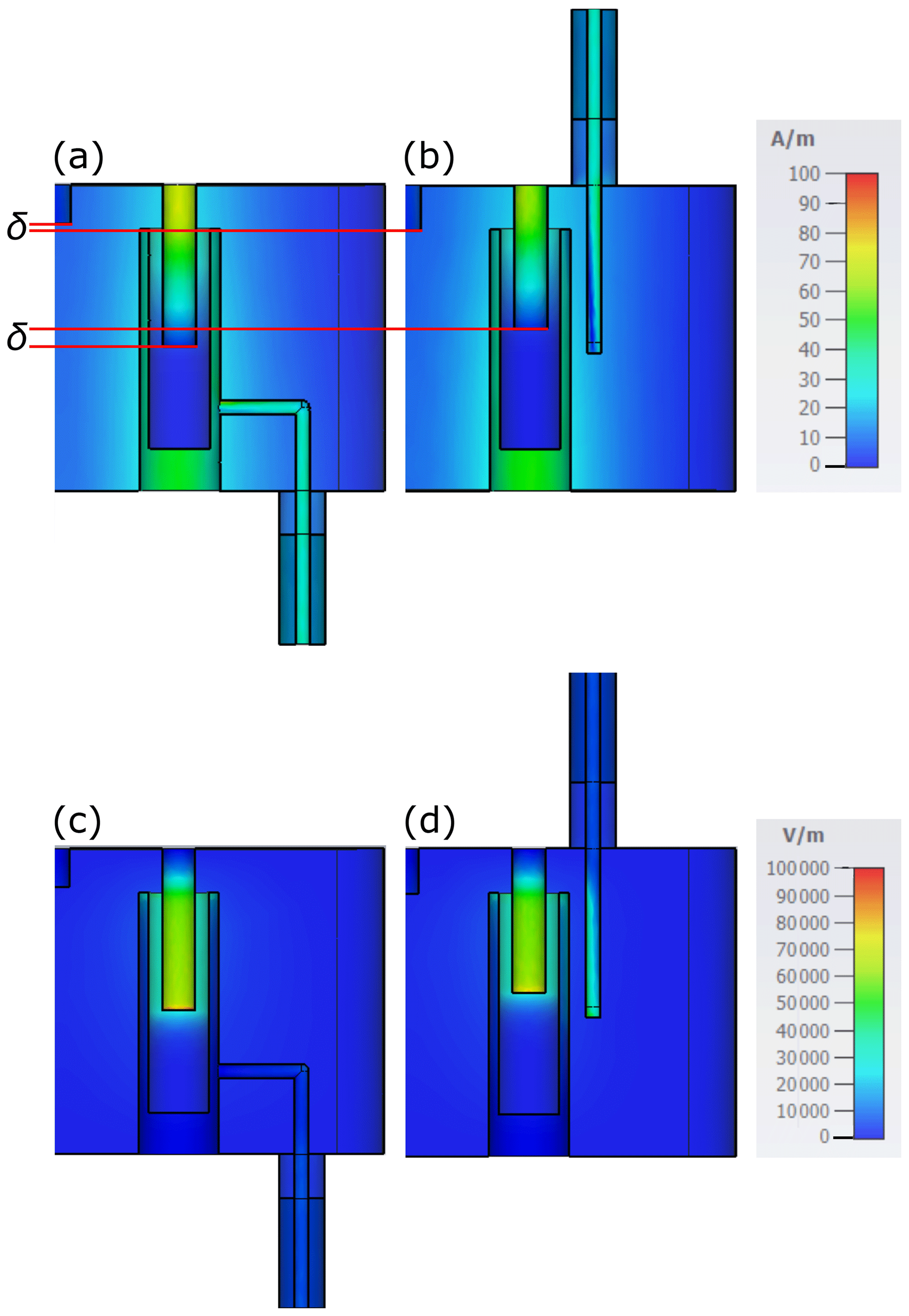
Figure 5 Maximum phasor amplitude at the center frequency: (a) current density for the inductive coupling; (b) current density for the capacitive coupling; (c) electric field for the inductive coupling; (d) electric field for the capacitive coupling. In panels (a) and (b), the straight red lines underline the different penetrations of tuning and coupling screws.

A qualitative explanation for the field maps follows. Reasoning in terms of transmission lines, for the inductive end coupling the voltage vanishes at the short circuit, and hence the associated electric transverse field vanishes too. At the same time, the current is maximum at the short circuit. Since the inductive coupling mainly excites the magnetic field, it must be only around the part of the resonator where the magnetic field is maximum, that is, near the lower end of the resonator. On the other hand, the capacitive end coupling is open-ended and it mainly excites the electric field. Therefore, the pin must be where the electric field is more intense, that is, at the top of the end resonator. The height h_p for both end couplings is less than $\mathit{\lambda }/\mathrm{4}$. Then, the input impedance at the coaxial cable–cavity transition seen looking inside the cavity presents an inductive (capacitive) imaginary component for the short-circuited (open-ended) inductive (capacitive) end coupling.

In addition, the capacitive end coupling requires a smaller penetration of the tuning screw and a greater penetration for the coupling screw than the inductive end coupling (Fig. 5a–b). In contrast, the three tuning screws of the three central resonators and the two coupling screws in between have penetrations almost unchanged over the two end couplings.

3.2.2 Filter response

Figure 6a shows the results for the measured response and the lossy synthesized response (Ness, 1998), that is, accounting for a finite Q_u. The agreement between curves is apparent. The measured unloaded quality factor averaged over resonators and end coupling types is $Q_{\mathrm{u}}=\mathrm{8}\times {\mathrm{10}}^{\mathrm{2}}$. This value is within the range foreseen for this kind of technology (Mansour, 2009). For the E1 Galileo bandwidth, the measured insertion loss at f₀ is 1.72 and 1.53 dB for the inductive and capacitive end couplings, respectively. The return loss is greater than 19 and 16 dB for the inductive and capacitive end coupling, respectively. Both measured responses have an insertion loss greater than 40 dB in the Iridium frequency range, as required by the specifications. For completeness, the group delay of the transmission coefficient is reported in Fig. 6b. There is no apparent difference between the curves, which proves the equality of the end couplings from an electrical point of view.

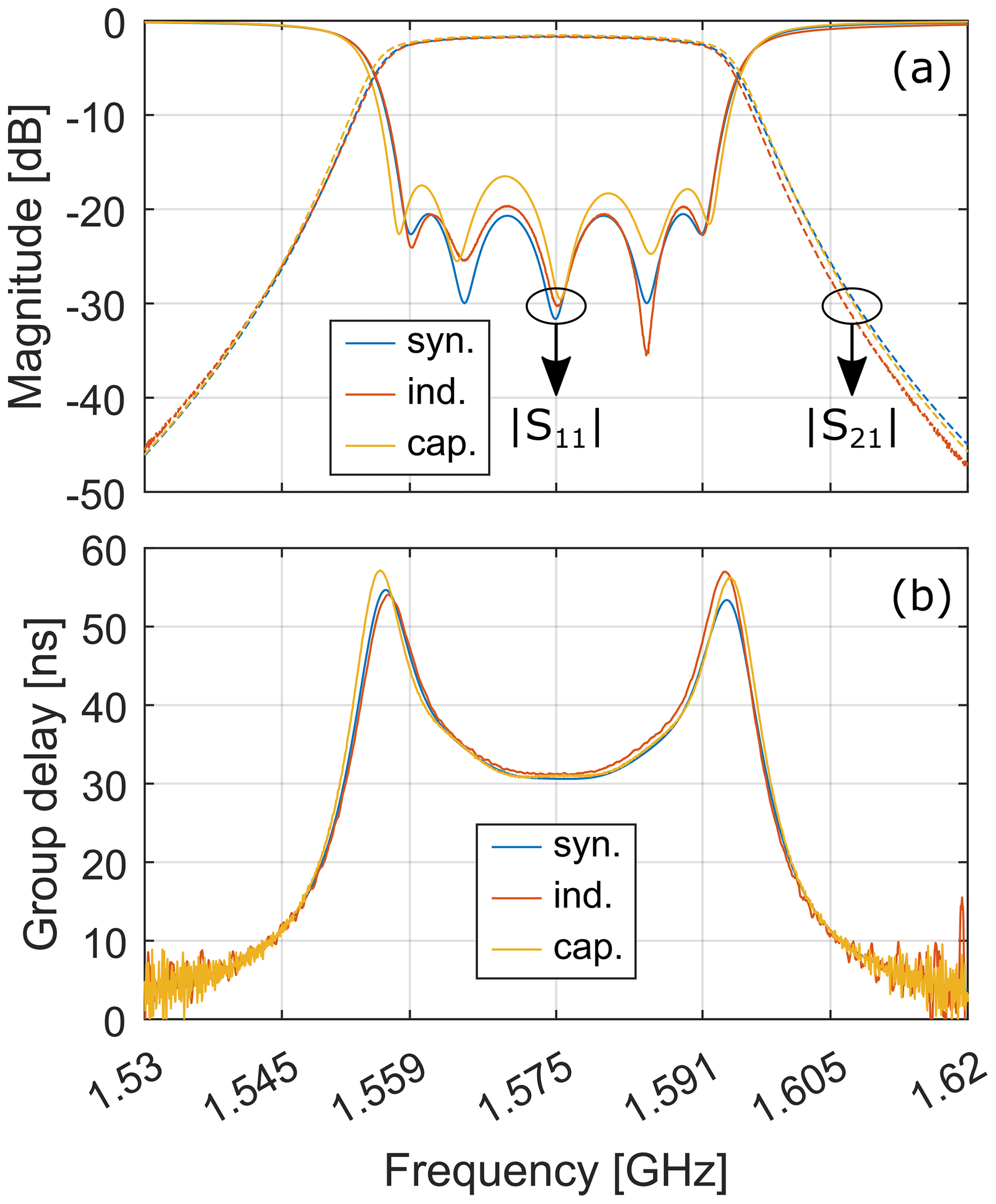
Figure 6 Lossy synthesized (syn.) and measured filter responses considering inductive (ind.) and capacitive (cap.) end couplings for the E1 Galileo band: (a) magnitude; (b) group delay of S₂₁.

The discrepancy between the synthesized and measured curves outside the passband is because the coaxial resonators approximate the lumped resonators of the synthesized response only around the center frequency (Zeng and Yu, 2024). It is then expected that far from this frequency there is a discrepancy between the lumped model and the distributed realization. This explains why the distributed realization presents spurious passbands. Observing the measured out-of-band response in Fig. 7, we notice that the insertion loss is greater than 40 dB up to 8.23 and 8.92 GHz for the inductive and capacitive end couplings, respectively. These frequencies are 5.22 and 5.66 times the center frequency of the E1 Galileo band. These values are close to the value of 5 foreseen by the theory (Yao et al., 1997).

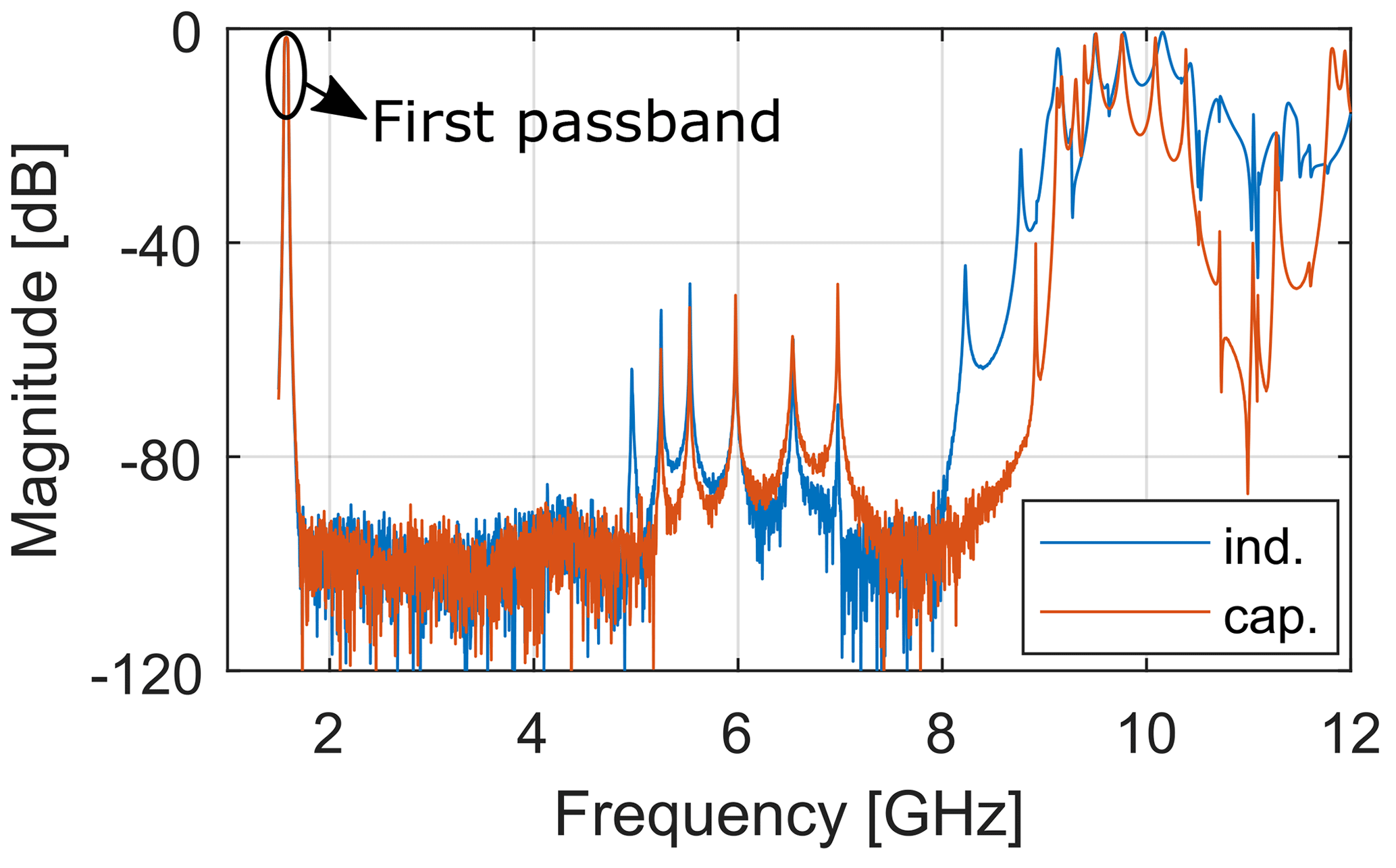
Figure 7 Wideband response of $\left|S_{\mathrm{21}}\right|$ considering inductive (ind.) and capacitive (cap.) end couplings. The filter is tuned at the E1 Galileo band.

To assess the capability of the filter to be tuned to other frequency ranges, the filter is also tuned on the Iridium band, and the results for the magnitude of the transmission and reflection coefficients, and the group delay are depicted in Fig. 8a and b, respectively. The realized bandwidth is 1605–1637.5 MHz (center frequency 1621.25 MHz) and it turns out to be wider than that of Iridium. It is not possible to have a narrower bandwidth because it is not possible to decrease the coupling between resonators. However, the insertion loss at the E1 Galileo band is greater than 20 dB. For completeness, independent of the type of end coupling the center frequency of the filter with the tuning and coupling screws extracted is about 2.655 GHz. This value then represents the maximum tuning frequency of the filter.

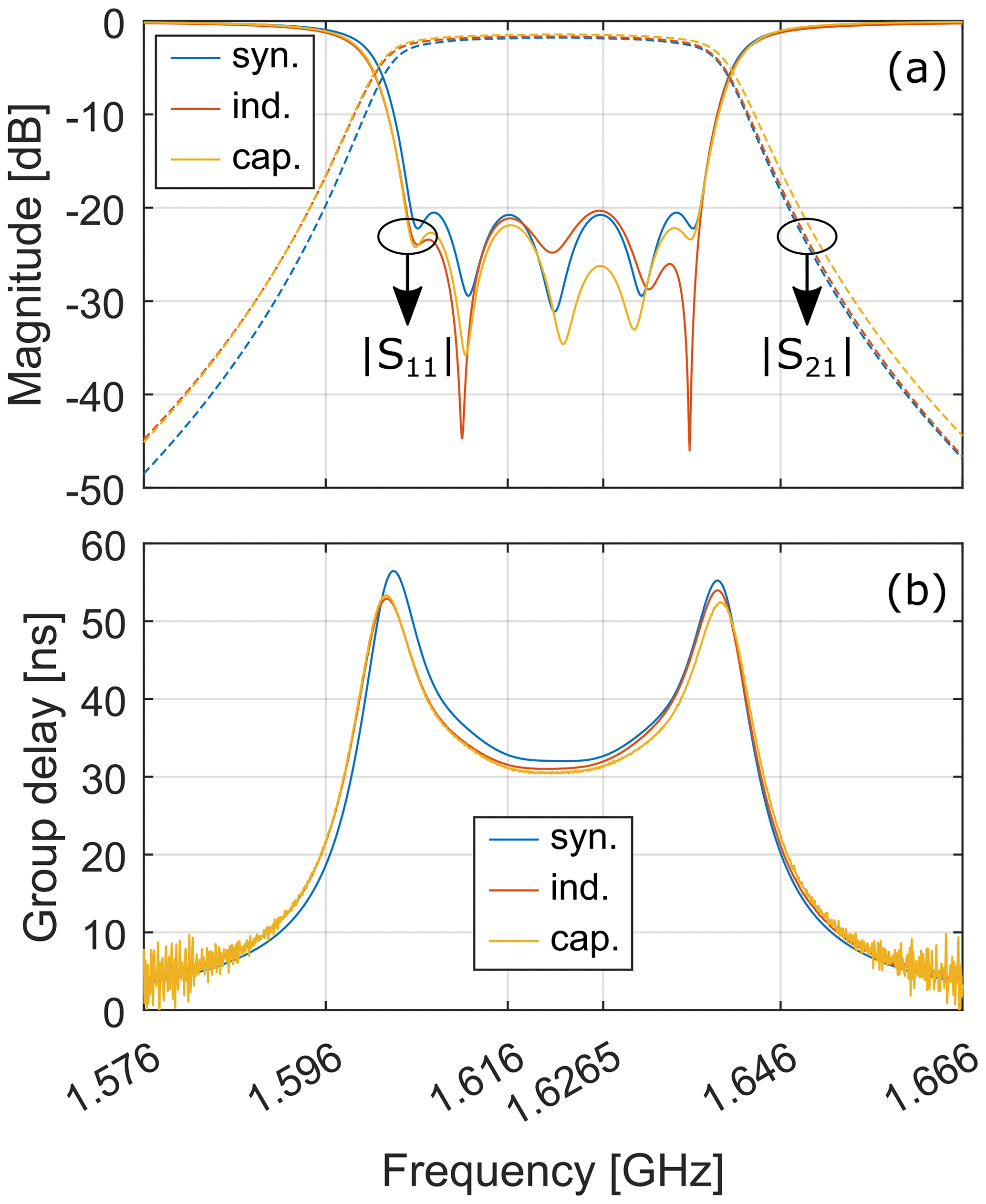
Figure 8 Lossy synthesized (syn.) and measured filter responses considering inductive (ind.) and capacitive (cap.) end couplings for the Iridium band: (a) magnitude; (b) group delay of S₂₁.

4 Conclusion

Inductive and capacitive end couplings in a combline cavity filter for the E1 Galileo band have been compared in terms of realized external quality factor, field maps, and filter response. The capacitive end coupling is easier to manufacture, and the external quality factor that it realizes is more sensitive to the pin height. The field maps have confirmed the expectation that the current density (electric field) plays a dominant role in the coupling mechanism of the inductive (capacitive) end coupling. Once the filter has been tuned to resonance, the two end couplings require different penetrations for the tuning and coupling screws of the input/output resonators. Overall, the realized filter has proven the effectiveness of the outlined design procedure for both types of end coupling.

As the next step, it would be of interest to investigate further the discrepancy between the simulated and measured curves for the external quality factor versus the pin height and to develop a theory-based fitting model for these curves.