From Schematics to Netlists – Electrical Circuit Analysis Using Deep-Learning Methods
Dennis Hemker
Jad Maalouly
Harald Mathis
Rainer Klos
Eranyan Ravanan
Within the project progressivKI, research is carried out to improve the analysis of schematics that depict an electrical circuit. Lots of manual efforts are necessary to validate a design, as schematics are handed in as image data. They neither follow a standard nor contain any meta information that can be obtained to automatically check certain conditions. Furthermore, even the visual representation of components like diodes, capacitors or resistors can differ depending on the design tool used.
In this paper, we present an approach to decompose the problem into three different parts and describe their current status: (i) detection of the components like resistors, capacitors, or diodes (ii) detection of lines and their junctions (iii) detection of textual data placed next to components (like voltage or resistance). For each of the given areas we employ deep-learning methods as a basis. The training data is provided by Microchip in the form of link-annotated PDFs. In a preprocessing phase, the data is programmatically scanned for useful information like component names and bounding boxes to pre-annotate them before human correction. The final step is to fuse all information from (i)–(iii) to obtain a netlist that can be automatically validated with given rules.
While most work has been carried out in (i) and (ii), a more general workflow including supportive tools has been established to extend our approach to PDFs from other design tools. The results show that recent deep-learning methods are capable of detecting components with a high accuracy given training data of good quality (no false labels).
- Article
(10314 KB) - Full-text XML
- BibTeX
- EndNote
Nowadays, electronic devices can be found in various applications and play an important role in people's everyday lives. From highly integrated mobile products like smartphones and laptops over public infrastructure, medical usage or as part of cars up to the aim of autonomous driving; electronics power many use-cases. Manufacturing such devices is a non-trivial task. Many factors like cost-effective component placement, electromagnetic compatibility issues or reuse and adaption of existing designs influence the development process.
However, one crucial representation of such systems is the schematic. It describes the components' (electrical) connectivity and functionality in a two-dimensional fashion. Having all information available in the design tool, it is possible to run checks and validations before a prototypical fabrication takes place.
From an industry perspective, schematics received from customers can be compared against their own reference designs, allowing detection of falsely integrated or parameterized components before production. Practical experiences show that aforementioned schematics are submitted as images (bitmaps) by customers lacking machine-readable information about component connections and properties. Furthermore, available design tools are shipped with their own set of symbol libraries not following a unique standard. As a result, design validation is often a manual, time-consuming and thus costly task.
Netlists are a commonly used format in electronic design. They can be of different complexities and representations, but also tailored down to a basic description of electronic components in the circuit and connected nodes (wires connecting pairs of components). A netlist can either be checked with scripts or potentially imported in tools like LTspice or Ngspice for further processing. As a conclusion, the depicted overall workflow can benefit from an automated, computer-based support.
In recent years, multiple approaches have been proposed to tackle similar problems. Most focus has been put on the detection of hand-written circuits. In Mohan et al. (2022) hand-drawn components are identified in two stages by geometrical properties or histogram of oriented gradients (HOG) features in combination with Support Vector Machine (SVM). Optical character recognition (OCR) trained on an extended MNIST dataset (Deng, 2012) is used to detect digits. Furthermore, for hand-written schematics, Huoming and Lixing (2019) utilize pixel distributions to segment components from lines. K-nearest neighbor is then applied on binarized component images to distinguish between 35 different classes. Rachala and Panicker (2022) compare deep-learning models SSD300 (Liu et al., 2016), YOLOv3 (Redmon and Farhadi, 2018) and YOLOv5 (Ultralytics, 2021) to detect five different components. Lines are obtained from Hough Transform after removing formerly detected components. The hand-written schematics used do not contain text. In Sertdemir et al. (2022) YOLOv5 is utilized to detect 13 different components in digital schematics (not hand-written). Lines are identified by Hough Transform whereas textual properties are derived from OCR and mapped to the closest nearby component (Euclidean distance). They provide an end-to-end software capable of generating netlists. A more general framework for hand-written sketches can be found in Altun and Nooruldeen (2019). Deep-learning techniques are used to detect digital logic circuit components and diagram structures. Custom designed Convolutional Neural Networks (CNN) of different depths are compared in Günay et al. (2020) to distinguish between four classes of hand-drawn components. They focus solely on the classification of isolated image patches from schematics. In Dey et al. (2021) a two-stage CNN is used to first classify hand-written circuit elements into one of four groups. Next, a group-specific classifier is applied enabling distinctiveness of 20 classes in total.
Most approaches described focus only on the processing of hand-written circuit diagrams. Furthermore, the number of component classes to be detected as well as the ability to detect text and lines varies. Lastly, most diagrams examined contain a small amount of components and lines but the usage of deep-learning methods shows promising results.
The rest of this paper is organized as follows. Section 2 explains the dataset used and how the overall problem is subdivided into the three subtasks component-, line- and text-detection. Section 3 examines the automatized extraction of ground truth information for each subtask. In the subsequent Sect. 4, respective deep-learning approaches and their performances are discussed. Section 5 shows how the deep-learning models' outputs are fused into a high-level representation again before concluding in Sect. 6.
In order to tackle the problem in more isolated ways, we propose to decompose the overall task into three sub-tasks:
-
Detection of electrical components including the type and respective bounding box. Identification of the line junctions is part of this task.
-
Detection of vertical and horizontal lines including their start and end points.
-
Detection and recognition of text including respective bounding boxes and the characters inside.
Finally, the geometrical information extracted by the three sub-tasks are assembled into a JavaScript Object Notation (JSON) file followed by a module combining them to a more abstract, high-level representation including connectivity. Different exporters can utilize the latter in order to generate netlists. The overall processing pipeline is depicted in Fig. 1.
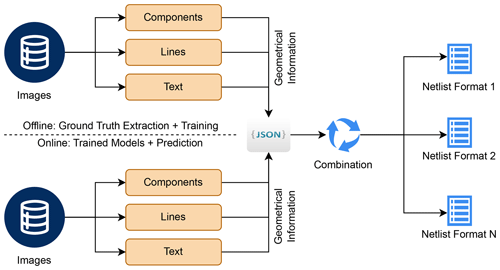
Figure 1Processing pipeline for training (offline) and prediction case (online) consisting of three parallel stages, fusion into a JSON file, inferring the connections by combining text, components and lines and finally netlist export.
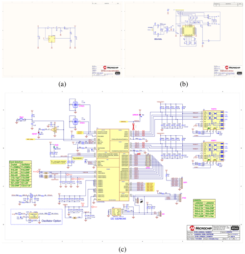
Figure 2Panel (a) represents a circuit with non-overlapping lines, small amount of components. Panel (b) shows overlapping lines and medium density of components. In panel (c), circuit with overlapping lines and high density of components is shown.
The collected dataset consists of 67 Portable Document Formats (PDFs) with a total number of 244 pages taking 95 MB disk space. These schematics depict electric circuits of different complexity made with the Altium Designer ©. By complexity, we refer to properties like overlapping vs. non-overlapping lines, text fragments which are clearly vs. non-clearly assignable to a specific component or the density of components. Example circuits can be found in Fig. 2.
Supportive text boxes, authoring information, embedded images and tables are ignored. Pages that do not contain a single electrical component are excluded completely which leads to a number of 164 usable pages. Note that the provided data is not artificially constructed but represents schematic designs currently used in industry by Microchip.
The provided PDFs are link-annotated and also contain Scalable Vector Graphics (SVG) data. For the training (offline) case, ground truth can be extracted, filtered and processed to necessary formats which reduces the efforts to manually label the images. In the prediction case (online), re-trained models generate the geometrical information required. Both mentioned stages produce a JSON file which is used in the combination component before exporting the schematic to a netlist. Additionally, the shared JSON format allows examinations of the combination module on the ground truth data. Subsequently, the same pipeline can ingest predictions.
Extraction of ground truth elements is done sequentially on-the-fly per page enabling images and labels to be converted and saved for each respective stage. All steps have in common that the PDF page is converted to a bitmap with 300 dpi for further task-specific processing. The dataset is generally split into train, test or validation sets specific to each stage. The architectural design allows for interruption before augmentation and splitting might be applied. Importing all automatically extracted ground truth data into LabelStudio (Tkachenko et al., 2022) for manual inspection, curation and extension is possible before feeding data back to the three stages. This approach can be considered semi-automated.
3.1 Component Detection
The schematics provided contain various symbols. As they are exported from Altium Designer ©, additional information about the components like textual description, category, part group or component type are stored in the PDF and shown while hovering over it in a PDF viewer.
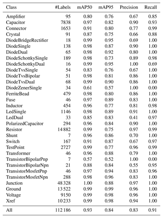
First, the PDF is scanned for its xref table. It can contain information about rectangles in the PDF, possible actions and references to JavaScript functions that execute on interaction. If the JavaScript xref contains a specific character, we collect the link ID together with the rectangle coordinates scaled relatively from the media box. In the next step, the PDF is opened in binary mode and processed line-wise. If the line contains one of the formerly collected link IDs and the keyword function, it is split by a delimiter. These splits are then compared against a list of regular expressions to obtain the ground truth class label for the component. This allows for applying search patterns to extract currently 32 classes as shown in Table 1.
Table 1Components mapped to exemplary regular expressions.
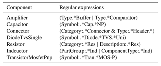
Excerpt of regular expressions used to obtain ground truth data for components.
Furthermore, junction points, ground symbols, voltage sources and cross references can also be found in the PDF. These are not provided with inline JavaScript functions, but can be identified by geometrical and color properties using the SVG data. Page is loaded using the community-developed Python library (Pdfminer.six, 2023) which enables iterating over SVG layout elements. In case of junctions, candidates are filtered by a specific stroke color. Next, if the SVG element consists of five points and the bounding box is nearly squared with a relative tolerance of 0.01, they are saved for later processing. Ground symbols are initially detected by a specific color and the type line. There exists two different shapes of ground symbols. One consists of five lines on top of each other shortening in length. The other again is depicted by five lines in a rake-like formation. As ground symbols consist of multiple, closely aligned lines, a density based clustering algorithm DBSCAN (Ester et al., 1996) is applied. The hyperparameters used are ϵ=15 (maximum distance to the point's neighbors) and min_samples = 5 (minimum amount of neighboring points) in the scikit-learn implementation (Pedregosa et al., 2011). Clusters consisting of exactly five lines are then fused given their labels and bounding boxes are calculated by minimum and maximum positions to frame the whole ground symbol. The voltage sources are depicted by two lines forming a T-shape of the same color as ground symbols. Again, the candidates are clustered as mentioned before but using a configuration of min_samples = 2 and rejecting clusters with not exactly two lines. The cross references are identified by SVG elements of type curve consisting of six or seven points and a specific stroke color. Additionally, candidates are checked for being not almost square, as cross references consist of one or two “arrows” to their left or right and are much wider than high. In total, 30 classes can be currently collected from the data set. Figure 3 shows an excerpt of extracted components.
3.2 Line Detection
The schematics only contain exact vertical and horizontal lines which represent the wires used to connect components. Although these lines can take multiple right-angled bends, we treat each straight part separately and recombine them later. The format of lines can then be described as:
For the set of all lines L the following condition holds true:
Line extraction is also done while iterating over all SVG objects in the PDF. Initially, the element is checked for a specific type (line or curve) and stroke color. Start and end points are saved in absolute coordinates. The image is binarized by thresholding it in the range [127,255] before saving using standard OpenCV functions (OpenCV, 2023). Figure 4 depicts extracted ground truth lines.
3.3 Optical Character Recognition
Again, while iterating per-page over all SVG objects, elements are checked for the type character ignoring color. Only text with an upright position is used because later OCR libraries can be given rotated images if necessary. Text in SVG data is provided per-character. In order to extract contiguous parts (words), again the density based clustering algorithm DBSCAN (Ester et al., 1996) is applied to group characters and digits. As the implementation used from scikit-learn (Pedregosa et al., 2011) works only on numbers, single characters are converted to their ordinal representation in Unicode. A custom distance function is implemented which takes into account the distance between top right and top left corner of two samples:
where x1, y1, x3, y3 are top left points and x2, y2, x4, y4 are bottom right. DBSCAN is applied with ϵ=3 and min_samples = 1. Clusters are then fused given their labels and bounding boxes are calculated by minimum and maximum positions. Ordinal cluster representation is reverted back to characters and text is saved together with bounding box coordinates. Figure 5 shows extracted ground truth data.
All subsequent experiments were carried out on a server providing up to eight NVidia RTX A5000 Desktop GPUs with 24GB. In all cases, no more than two GPUs were used for one training pipeline. The code is integrated in a modular way so it can run in a non-interactive mode on the servers implementing an architecture described in Hemker et al. (2023).
4.1 Component Detection
Initially, first experiments were carried out by using the well-known object detector SSD300 (Liu et al., 2016). As it accepts only images of size 300×300 pixels, input data needed to be scaled down to the proper resolution. Original images extracted from the PDF typically have a size up to 5096×3300 pixels. Scaling them as a whole to the required resolution leads to bad classification performance because of poor quality. Components are relatively small compared to the overall image size so downscaling blurred them. To overcome this issue, a different approach was applied. The image was rasterized into overlapping tiles of size 300×300 pixels and then passed to the SSD300 training pipeline. It led to better detection results but a post-processing step using non-maximum suppression to filter out duplicate bounding boxes in the tiles was necessary. All in all, the prediction results were more accurate but at the cost of longer calculation times. Taking into account the future requirement to detect integrated circuits in the images which can span more than 300×300 pixel tiles, a different solution was required.
Research on more recent object detection models and promising results from related work papers lead to YOLOv7 (Wang et al., 2023) which comes with faster inference and improved performance on the COCO dataset (Lin et al., 2014). In order to fine-tune the YOLOv7 on our schematic dataset, an augmentation pipeline is used to generate more samples for training. First, images are converted to grayscale (for avoiding color dependencies) and then fed into a composed augmentation pipeline employing Albumentations (Buslaev et al., 2020). It contains two steps:
-
Cropping random chunks of the input image with size 800×800 pixels and probability p=1.0.
-
Random rotation of the chunks by either zero or multiples of 90∘ with probability p=0.5.
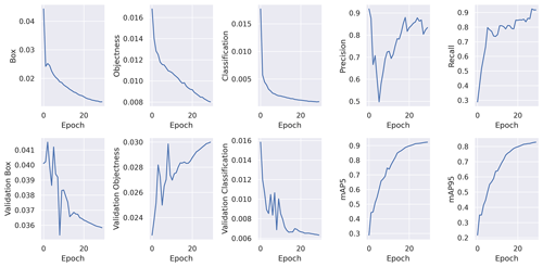
Figure 6Available training and validation metrics for YOLOv7. The losses are heavily decreasing until the tenth epoch and keep lowering until epoch 30. Scores like precision, recall and mAP are increasing and flatten after epoch 20. It is notable that validation objectness is alternating but generally increasing. This can either be an indicator for the start of overfitting or for fragments of components (not fully visible) in the validation set which are not labeled. They count as background and impact the aforementioned score.
Only fully visible bounding boxes in augmented images are accepted. Applying augmentation with the given pipeline 500 times per input image yields a total number of 59 706 images for fine-tuning alongside their ground truth data (564 786 annotations) in the YOLO-specific format. Training is performed for 30 epochs, a batch size of 4, pre-trained model weights and the default configuration file yolov7/cfg/training/yolov7.yaml and hyperparameter file yolov7/data/hyp.scratch.p5.yaml found in the original Github repository. Data is split into 60 % train, 20 % validation and 20 % test sets. The metrics and losses used in the further course are briefly explained in the following, whereby TP denotes the number of true positives, TN the true negatives and FP the false positives.
-
Precision: The ratio of true positives to all positive predictions.
-
Recall: Measures how many of the positive instances were identified as such.
-
Mean average precision (mAP): Taking into account precision, recall and the intersection over union (IoU) to evaluate performance. If the IoU is above a given threshold, predictions are considered as positive. Variations of the aforementioned threshold are reflected in the mAP50-95 values, respectively.
-
Box: Loss that takes into account the error between predicted and actual bounding box coordinates.
-
Objectness: Loss of how good the model is able to identify the presence of an object in an image.
-
Classification: Loss to quantify the error of assigning the correct label (class) to a bounding box.
For further loss descriptions see Wang et al. (2023) and on how the mAP is calculated (using intersection of union for bounding boxes), see Henderson and Ferrari (2017). Figure 6 depicts loss and scoring behavior during training. Until epoch 20, the losses significantly decrease while mean average precision (mAP) in addition to precision and recall rise. It is notable that the validation objectness is alternating but rising during training. It could indicate component symbols in the validation dataset which are not labeled as such, leading to false background detections or the early start of overfitting.
Results of the test set are shown in Table 2. It can be seen that the overall detection performance is quite high (mAP95 ≥ 0.73 for all classes except the DiodeZenerSingle and TransistorBipolarPnp). However, some components like Crystal, Shunt and different Diodes or Transistors are underrepresented in the datasets compared to Resistor, Capacitor, Junction and Ground. In particular, the classes DiodeZenerSingle and TransistorBipolarPnp show a bad performance. The total number of samples found in the train and test sets is quite low, but this is also the case for other, better performing classes. A possible explanation could be a failure in the extraction of pre-annotations. This requires a manual inspection before augmentation. Nevertheless, the model seems to learn their visual properties and having more images with these classes available could lead to more robust results. In the next steps, classes will be extended by more components like integrated circuits.
4.2 Line Detection
Initial tests were performed with the well-known probabilistic Hough Transform (Kiryati et al., 1991). Although it can lead to slightly worse detections compared to classical Hough Transform, calculation speed is much higher. In a qualitative investigation with different algorithm parameters implemented in OpenCV (OpenCV, 2023), resulting line detections are mostly cluttered, noisy and duplicate. Figure 7 shows an example line detection with probabilistic Hough Transform parameters ρ=1 (distance resolution of the accumulator in pixels), (angle resolution of the accumulator in radians), threshold = 10 (minimum number of votes required for a line), minLineLength = 10 (minimum line length), maxLineGap = 50 (maximum allowed gap between points to still treat them as the same line).
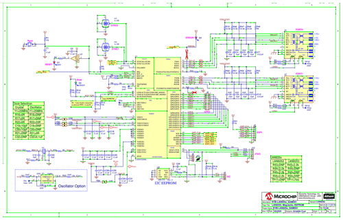
Figure 7Cropped view of lines calculated with probabilistic Hough Transform from Fig. 2c. Black dots show start and end points. Lines are colored green.
Lines are in some places detected on both gradient sides of the original line boundaries (one at the top, one at the bottom). Gaps are present in many cases and false positives are detected e.g. within integrated circuit shapes. Different parameters lead to the inclusion of more line candidates at the cost of finding digits or parts of characters and components. As fine-tuning these parameters for the whole or even new datasets is a nearly impossible task, research on the latest models capable of detecting lines leads to L-CNN (Zhou et al., 2019). The authors state to outperform previous state-of-the-art line detectors with their model. The implementation provided via Github repository allows for fine-tuning the L-CNN on custom data. In the first step, binarized images are stored in a folder wireframe_raw/images (required). Next to it, two JSON files (training and validation) contain a list of image file names alongside the start and end points of the respective lines. The data is split into 80 % train and 20 % validation set. The L-CNN pipeline automatically creates a folder called wireframe and places augmented images. They include random flips and rotations while the resolution is scaled down to have squared dimensions leading to a total number of 496 images with 191 004 lines as the training set. The validation set is not augmented yielding a total number of 31 images containing 7843 lines. For training, default wireframe.yaml configuration is applied but the number of epochs is set to 300. Zhou et al. (2019) propose a new evaluation metric called structural average precision (sAP) which is inspired by the mAP for object detection tasks. The strictness of this metric is controlled with a user-defined threshold .
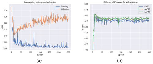
Figure 8Panel (a) shows the training and validation loss of L-CNN for 300 epochs. The loss combines multiple metrics for junction and line candidate heat maps. Panel (b) shows the different sAP scores for validation set.
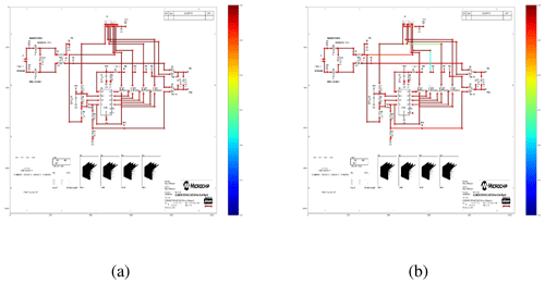
Figure 9Randomly taken example schematic from the validation set at the best performing epoch. Panel (a) shows the ground truth data. Panel (b) depicts line predictions. Most lines show a high confidence score. A small amount of lines is falsely proposed as they span across multiple junction points.
Figure 8 shows the loss curve for training and validation next to the aforementioned sAP scores for the validation set. Around epoch 10, the validation loss reaches a minimum while training loss still reduces. This can be an indicator for the model to start overfitting the data. Furthermore, all sAP scores show the best performance around the mentioned epoch. Default L-CNN scripts from Github save the best performing model checkpoint together with the latest one. An example schematic showing both ground truth and proposed predictions can be found in Fig. 9. Compared to the classical approaches like probabilistic Hough Transform, lines appear less noisy and are not chunked by gaps. Additionally, there are no duplicate lines on the bottom/top gradient sides. However, in parts with high density of closely neighboring lines, not all candidates are detected. A possible reason can be the automatized downscaling of the schematic during L-CNN pipeline. The loss in resolution could potentially lead to blurred separations. In a post-processing step, predicted lines that are not fulfilling condition (1) up to a small tolerance are filtered out. Next steps include analysis of non-detected lines and possible mitigations. Blurrings in dense areas caused by downscaling can potentially be enhanced by applying pre-processing methods.
4.3 Optical Character Recognition
A first qualitative investigation was carried out using three prominent OCR libraries PaddleOCR (Du et al., 2020), docTR (Mindee, 2021) and EasyOCR (JaidedAI, 2023). All of them provide easy-to-use interfaces for loading an image and scanning it for text. Additionally, they take care for necessary pre-processing steps like binarization or downscaling if required. Best results without changing any of the possible parameters using random schematics were provided by EasyOCR. Initial results can be seen in Fig. 10. The text next to the capacitors is precisely detected and separated while next to resistors the characters are combined into a bigger horizontal box spanning over the component symbols. However, especially small digits representing the pin numbers are mostly not detected which is the case for all three libraries.
EasyOCR allows for fine-tuning its detection model, namely CRAFT (Baek et al., 2019). A training pipeline is provided within the Github repository. We used the default configuration and started fine-tuning with a model checkpoint trained on both SynthText (Gupta et al., 2016) and ICDAR 2015 (Karatzas et al., 2015) dataset. Augmentations like rotations, crops or flips are handled by the pipeline itself. Data is split in the same ratio as line detection to 80 % train and 20 % validation sets. In total, 124 images with 46 498 text boxes are used for training while validation includes 31 images and 13 075 text boxes. We run evaluations every 200 epochs while training is set to 8000 epochs. Default configuration file trainer/craft/config/custom_data_train.yaml is used with adaptions to data set locations and number of epochs.
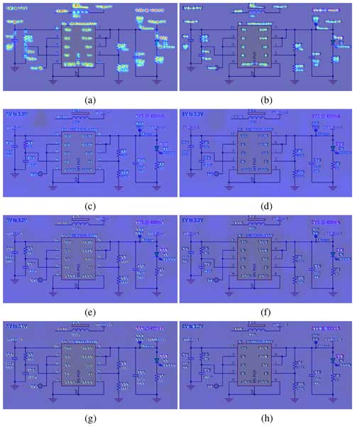
Figure 11Cropped view of detection heatmaps for exemplary schematic. Panel (a) shows the heatmap for character candidates. Heatmap (b) depicts the connectivity between characters (grouping them to words), both calculated by default pre-trained CRAFT. The model particularly finds characters and parts of components, but pin numbers do not show a high response in both cases. After 400 epochs, panels (c) and (d) indicate lower response in formerly hot regions. Validation at epoch 2000 in panels (e) and (f) shows a higher response again, now including pin numbers. Panels (g) and (h) only indicate small improvements around the pin numbers after 7800 epochs, but text consisting of multiple characters or digits shows higher scores.
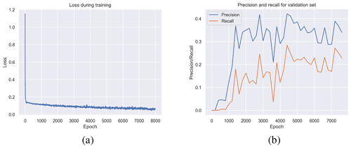
Figure 12Panel (a) shows the loss during training. After a few epochs, it is strongly decreasing and keeps lowering until final epoch 8000. Precision and recall curves in panel (b) show best performance at around 3000 and 4500 epochs. Considering the still decreasing loss, increasing the number of epochs could lead to better performance.
Figure 11 shows exemplary validation results during training after 0 (default pre-trained weights), 400, 2000 and 7800 epochs. The CRAFT model seems to quickly lose its previous capabilities as the detection candidate heatmaps decrease, but later steps show an increased response on pin number digits. Taking into account the precision and recall during validation together with the training loss, it can be seen that the loss is still decreasing while validation metrics improve. As the model adapts to new data, predicted text candidates are below the detection threshold so no bounding boxes are obtained. Further epochs of training cause more valid bounding boxes to be proposed by the model, leading to increasing precision and recall values. However, after 8000 epochs, heatmaps at already intense places are not as strong as the initial ones. Taking into account the precision and recall curves in Fig. 12, training progress could be flattening. Further investigations include increasing the number of epochs to see if heatmap activity resembles the original performance in all regions while precision and recall rise. Please note that the presented studies are only about text detection and recognition can be examined afterwards. Alternatives can be further image pre-processing strategies and augmentation in addition to replacing the pipeline with a different architecture.
Finally, the information predicted by the three presented models are fused into a single JSON description containing components, lines and text alongside their bounding boxes or start and end points in relative coordinates. Furthermore, each detection is assigned a unique identifier and metadata can be added if required.
We refer to these raw detections as geometrical primitives. In order to infer high-level information from them, components are matched against lines. Additionally, the detected text is mapped to its closest components. Both alignments are done by calculating the Euclidean distance from the bounding box center coordinates. First qualitative results show the general feasibility of this approach. However, as text placement does not follow a specific scheme (it can be visible on any of the four sides around the component), wrong matches are obtained. Even from a human perspective, it is hard to assign particular text placements to components with high confidence. Another challenge is the handling of non-closed lines. These are linked to external connections that are not part of the regular electrical component classes. However, it is expected that not all cases can be handled automatically. As the fusion strategy depends on parameters like the distance threshold and selection of reference points used for calculations, a human in the loop could select appropriate values per schematic on demand.
Connections of text, components and lines are stored in an internal, more abstract format. Given this high-level representation, various netlist exporters can be implemented in the future. Possible variants are simple ones following a SPICE layout, e.g. CC8 0 NetC8_2 100pF depicting capacitor C8 is connected to ground (0) and net NetC8_2 having value 100pF. More complex structures include the Electronic Design Interchange Format (EDIF). Finally, exported structures can serve as input for validation checks and other pipelines.
In this paper, an approach to reconstruct connectivity information of electrical circuits from schematic images is presented. First, the problem is decomposed into three parts, namely component, line, and text detection. For each of these stages, deep-learning models are selected and applied to solve the task. Using a publicly available, industry relevant dataset based on Altium Designer © schematics, ground truth information can be obtained by raw PDF parsing and SVG processing. Both ground truth data and predictions can be fused into a JSON format containing geometrical primitives. In the next step, high-level representation is inferred to connect components, lines and text. Finally, the proposed architecture allows to interface netlist exporters here which can transform this representation to formats of different complexity. First tests show promising results, especially for component and line detection stages.
However, the next steps include adding integrated circuits to the list of detectable components. Our current analysis shows that they do not share common properties in the PDF link-annotations and thus need to be labeled manually. Further work is required to detect the orientation of components which is necessary for analyzing pin connections. Moreover, the text detection pipeline requires further analysis, especially because of the small pin numbers to be detected. Additionally, as the current geometrical primitive combination is checked qualitatively by human inspection, the acquisition of ground truth data on the connectivity level (netlists) is essential for comparable metrics in the final reassembly stage. It is expected that the fusion process requires small adjustments by a human before exporting to netlists. However, the data used can be taken from other design tools to train from scratch or fine-tune existing models. Therefore, the method presented can be used as a framework.
Due to project restrictions, source code is not published.
The link-annotated PDFs were taken from the publicly available schematics by Microchip. The dataset is hosted internally on Fraunhofer infrastructure and persisted. Readers can contact the correspondence author or any other of the named authors to get access to the dataset.
DH provided graphical and textual contributions and programmed together with JM the computer code. Conceptual design, discussion and analysis of results was done by DH, JM, HM, RK and ER. RK and ER further composed the dataset and provided domain knowledge.
The contact author has declared that none of the authors has any competing interests.
Publisher's note: Copernicus Publications remains neutral with regard to jurisdictional claims made in the text, published maps, institutional affiliations, or any other geographical representation in this paper. While Copernicus Publications makes every effort to include appropriate place names, the final responsibility lies with the authors.
This article is part of the special issue “Kleinheubacher Berichte 2023”. It is a result of the Kleinheubacher Tagung 2023, Miltenberg, Germany, 26–28 September 2023.
This research has been supported by the Bundesministerium für Wirtschaft und Klimaschutz (grant nos. 19A21006D, 19A21006L, and 19A21006Q).
This paper was edited by André Buchau and reviewed by two anonymous referees.
Altun, O. and Nooruldeen, O.: SKETRACK: stroke-based recognition of online hand-drawn sketches of arrow-connected diagrams and digital logic circuit diagrams, Sci. Programming, 2019, 1–17, https://doi.org/10.1155/2019/6501264, 2019. a
Baek, Y., Lee, B., Han, D., Yun, S., and Lee, H.: Character Region Awareness for Text Detection, 2019 IEEE/CVF Conference on Computer Vision and Pattern Recognition (CVPR), 15–20 June 2019, Long Beach, USA, IEEE, https://doi.org/10.1109/CVPR.2019.00959, 2019. a
Buslaev, A., Iglovikov, V. I., Khvedchenya, E., Parinov, A., Druzhinin, M., and Kalinin, A. A.: Albumentations: Fast and Flexible Image Augmentations, Information, 11, 125, https://doi.org/10.3390/info11020125, 2020. a
Deng, L.: The MNIST Database of Handwritten Digit Images for Machine Learning Research [Best of the Web], IEEE Signal Proc. Mag., 29, 141–142, https://doi.org/10.1109/MSP.2012.2211477, 2012. a
Dey, M., Mia, S. M., Sarkar, N., Bhattacharya, A., Roy, S., Malakar, S., and Sarkar, R.: A two-stage CNN-based hand-drawn electrical and electronic circuit component recognition system, Neural Comput. Appl., 33, 13367–13390, 2021. a
Du, Y., Li, C., Guo, R., Yin, X., Liu, W., Zhou, J., Bai, Y., Yu, Z., Yang, Y., Dang, Q., and Wang, H.: PP-OCR: A Practical Ultra Lightweight OCR System, CoRR, arXiv [preprint], https://doi.org/10.48550/arXiv.2009.09941, 21 September 2020. a
Ester, M., Kriegel, H.-P., Sander, J., and Xu, X.: A density-based algorithm for discovering clusters in large spatial databases with noise, in: KDD'96: Proceedings of the Second International Conference on Knowledge Discovery and Data Mining, 2–4 August 1996, Portland, USA, AAAI Press, vol. 96, 226–231, https://dl.acm.org/doi/proceedings/10.5555/3001460 (last access: 28 November 2024), 1996. a, b
Günay, M., Köseoğlu, M., and Yıldırım, Ö.: Classification of hand-drawn basic circuit components using convolutional neural networks, in: 2020 International Congress on Human-Computer Interaction, Optimization and Robotic Applications (HORA), 26–28 June 2020, Ankara, Turkey, IEEE, 1–5, https://doi.org/10.1109/HORA49412.2020.9152866, 2020. a
Gupta, A., Vedaldi, A., and Zisserman, A.: Synthetic data for text localisation in natural images, in: Proceedings of the IEEE conference on computer vision and pattern recognition, 27–30 June 2016, Las Vegas, USA, IEEE, 2315–2324, https://doi.org/10.1109/CVPR.2016.254, 2016. a
Hemker, D., Kreutter, S., and Mathis, H.: On Reducing Complexity in AI Pipelines: Modularisation to Retain Control, ERCIM News 133, ERCIM EEIG, BP 93, Sophia Antipolis Cedex, France, https://ercim-news.ercim.eu/images/stories/EN133/EN133-web.pdf (last access: 28 November 2024), 2023. a
Henderson, P. and Ferrari, V.: End-to-end training of object class detectors for mean average precision, in: Computer Vision–ACCV 2016: 13th Asian Conference on Computer Vision, Taipei, Taiwan, 20–24 November 2016, Revised Selected Papers, Part V 13, Springer, 198–213, https://doi.org/10.1007/978-3-319-54193-8_13, 2017. a
Huoming, Z. and Lixing, S.: Research on K nearest neighbor identification of hand-drawn circuit diagram, J. Phys. Conf. Ser., 1325, 012233, https://doi.org/10.1088/1742-6596/1325/1/012233, 2019. a
JaidedAI: EasyOCR, GitHub [code], https://github.com/JaidedAI/EasyOCR (last access: 20 January 2024), 2023. a
Karatzas, D., Gomez-Bigorda, L., Nicolaou, A., Ghosh, S., Bagdanov, A., Iwamura, M., Matas, J., Neumann, L., Chandrasekhar, V. R., Lu, S., Shafait, F., Uchida, S., and Valveny, E.: ICDAR 2015 competition on Robust Reading, in: 2015 13th International Conference on Document Analysis and Recognition (ICDAR), 23–26 August 2015, Nancy, France, 1156–1160, https://doi.org/10.1109/ICDAR.2015.7333942, 2015. a
Kiryati, N., Eldar, Y., and Bruckstein, A. M.: A probabilistic Hough transform, Pattern Recogn., 24, 303–316, 1991. a
Lin, T.-Y., Maire, M., Belongie, S., Hays, J., Perona, P., Ramanan, D., Dollár, P., and Zitnick, C. L.: Microsoft coco: Common objects in context, in: Computer Vision–ECCV 2014: 13th European Conference, Zurich, Switzerland, 6–12 September 2014, Proceedings, Part V 13, Springer, 740–755, https://doi.org/10.1007/978-3-319-10602-1_48, 2014. a
Liu, W., Anguelov, D., Erhan, D., Szegedy, C., Reed, S., Fu, C.-Y., and Berg, A. C.: Ssd: Single shot multibox detector, in: Computer Vision–ECCV 2016: 14th European Conference, Amsterdam, the Netherlands, 11–14 October 2016, Proceedings, Part I 14, Springer, 21–37, https://doi.org/10.1007/978-3-319-46448-0_2, 2016. a, b
Mindee: docTR: Document Text Recognition, GitHub [code], https://github.com/mindee/doctr (last access: 15 January 2024), 2021. a
Mohan, A., Mohan, A., Indushree, B., Malavikaa, M., and Narendra, C.: Generation of Netlist from a Hand drawn Circuit through Image Processing and Machine Learning, in: 2022 2nd International Conference on Artificial Intelligence and Signal Processing (AISP), 12–14 February 2022, Vijayawada, India, IEEE, 1–4, https://doi.org/10.1109/AISP53593.2022.9760577, 2022. a
OpenCV: Open Source Computer Vision Library, GitHub [code], https://github.com/opencv/opencv (last access: 28 November 2024), 2023. a, b
Pdfminer.six: Pdfminer.six, GitHub [code], https://github.com/pdfminer/pdfminer.six (last access: 16 January 2024), 2023. a
Pedregosa, F., Varoquaux, G., Gramfort, A., Michel, V., Thirion, B., Grisel, O., Blondel, M., Prettenhofer, P., Weiss, R., Dubourg, V., Vanderplas, J., Passos, A., Cournapeau, D., Brucher, M., Perrot, M., and Duchesnay, E.: Scikit-learn: Machine Learning in Python, J. Mach. Learn. Res., 12, 2825–2830, 2011. a, b
Rachala, R. R. and Panicker, M. R.: Hand-drawn electrical circuit recognition using object detection and node recognition, SN Computer Science, 3, 244, https://doi.org/10.1007/s42979-022-01159-0, 2022. a
Redmon, J. and Farhadi, A.: Yolov3: An incremental improvement, arXiv [preprint], https://doi.org/10.48550/arXiv.1804.02767, 8 April 2018. a
Sertdemir, A. E., Besenk, M., Dalyan, T., Gokdel, Y. D., and Afacan, E.: From Image to Simulation: An ANN-based Automatic Circuit Netlist Generator (Img2Sim), in: 2022 18th International Conference on Synthesis, Modeling, Analysis and Simulation Methods and Applications to Circuit Design (SMACD), 12–15 June 2022, Villasimius, Italy, IEEE, 1–4, https://doi.org/10.1109/SMACD55068.2022.9816254, 2022. a
Tkachenko, M., Malyuk, M., Holmanyuk, A., and Liubimov, N.: Label Studio: Data labeling software, GitHub [code], https://github.com/heartexlabs/label-studio (last access: 20 November 2024), 2022. a
Ultralytics: YOLOv5: A state-of-the-art real-time object detection system, https://docs.ultralytics.com (last access: 16 January 2024), 2021. a
Wang, C.-Y., Bochkovskiy, A., and Liao, H.-Y. M.: YOLOv7: Trainable bag-of-freebies sets new state-of-the-art for real-time object detectors, in: Proceedings of the IEEE/CVF Conference on Computer Vision and Pattern Recognition, 18–22 June 2023, Vancouver, Canada, 7464–7475, https://doi.org/10.1109/CVPR52729.2023.00721, 2023. a, b
Zhou, Y., Qi, H., and Ma, Y.: End-to-end wireframe parsing, in: Proceedings of the IEEE/CVF International Conference on Computer Vision, 27 October–2 November 2019, Seoul, South Korea, IEEE, 962–971, https://doi.org/10.1109/ICCV.2019.00105, 2019. a, b
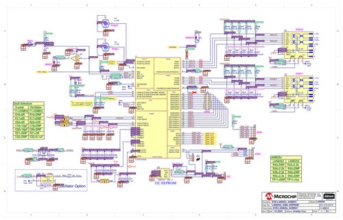
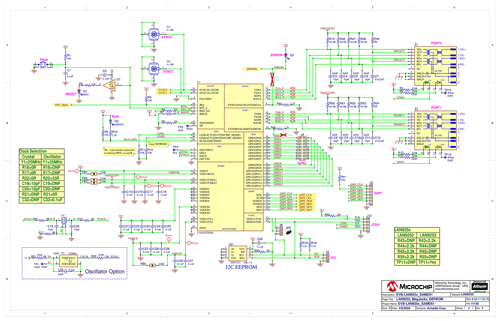
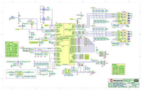
With the help of deep-learning methods, components, lines and text can be extracted from these bitmaps.
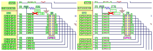
Fusing these detections, the electrical circuit can be reconstructed and serve as an input for further validation routines.


