A review of orthogonal waveforms for spaceborne Multiple-Input Multiple-Output Synthetic Aperture Radar

Spaceborne Multiple-Input Multiple-Output Synthetic Aperture Radar (MIMO-SAR) overcomes fundamental shortcomings of state-of-the-art SAR, such as the trade-off between swath width and spatial resolution, and offers a greater agility of the antenna beam steering. In addition, MIMO-SAR enables a wide variety of new operation and acquisition modes, such as the High-Resolution Wide-Swath (HRWS) mode. One demanding requirement in this subject is to design separable orthogonal waveforms which optimize the overall imaging performance. In the case of a SAR system, this is not an easy task due to the nature of the imaged scene consisting of a multitude of point and distributed targets. This paper summarizes the most promising waveforms in the literature and analyzes them in detail. The selected waveforms are investigated for the first time with respect to their use in SAR using the ambiguity function. As a conclusion, a catalogue of important waveform performance parameters and an ambiguity function analysis are provided, to support the modern MIMO-SAR designer in the form of decision rules for the optimal waveform selection.

1 Introduction

One of the key challenges in MIMO-SAR is channel separation on receive (Krieger et al., 2012; Krieger, 2014). In a MIMO-SAR system, the transmitted waveform signals overlap, creating a multiplicity of channels within the transmit mode, while the echo signals at the receive channels are acquired individually and simultaneously. To be able to separate all possible channel combinations in post-processing, several approaches can be considered. Basically, MIMO systems require orthogonal waveforms to allow the transmitted waveforms to be fully separable at the receiver. Nowadays, MIMO systems, methodologies, and processing strategies are well established the field of communications. For radar applications, however, these features need to be adapted accordingly.

One typical application example of MIMO-SAR are simultaneous fully polarimetric acquisitions (Krieger et al., 2008). In conventional fully polarimetric SAR, the radar transmits in horizontal and vertical polarization in an interleaved mode. Both polarizations are received and recorded simultaneously. Thus, to keep the sampling rate the same, the pulse repetition frequency PRF has to be increased by a factor of two, which decreases the swath width by the same factor. In contrast, in fully polarimetric MIMO-SAR, the transmitter simultaneously transmits orthogonal signals in both polarizations. At the receiver, two separate channels in orthogonal polarization states simultaneously receive horizontal and vertical polarized signals. This approach allows for the simultaneous measurement of all four parameters of the scattering matrix (HH, HV, VH, VV). Unlike conventional fully polarimetric SAR, the use of MIMO preserves the PRF, maintaining both resolution and swath-width. However, this necessitates the use of orthogonal waveforms. Another possible field of application is MIMO-SAR across-track interferometry. The use of multiple channels allows multiple virtual antenna phase centers and thus multiple simultaneous interferometric baselines. This allows larger baselines for an improved height accuracy while solving for phase ambiguities with short baselines. In addition, a direct phase synchronization of the multistatic radar system is possible. Further application examples can be found in Krieger et al. (2016), Tebaldini et al. (2024).

The rapid increase in data volumes in communication systems has intensified research into advanced techniques for separating superimposed signals while avoiding interference with other channels. In various communication applications, such as radio, television, telecommunications, or satellite navigation, multiplexing techniques are used to distinguish between transmitters. These techniques exploit channel capacity by using information about space (beam-forming), polarization, frequency, time, or correlation (Ohm and Lueke, 2004; Haykin and Moher, 2009). More specifically, we distinguish between Space Division Multiplex (SDM), Polarization Multiplex (PM), Frequency Division Multiplex (FDM), Time Division Multiplex (TDM) and Code Division Multiplex (CDM)¹.

With respect to MIMO radars, the information about the channel is of interest and the transmitted signals are known, whereas in communications the users are usually interested in the information content of the transmitted signal. Because the goal is different, it is necessary to adapt the techniques from communications to radars. As explained in the first section of this paper, the waveforms for MIMO radar and MIMO-SAR have certain requirements that make it more difficult to separate the individual signals and channels. The challenge of separating individual signals and channels in MIMO radar systems requires novel approaches tailored to radar-specific requirements. At the same time, it is important to distinguish between high-resolution imaging MIMO radar (e.g. MIMO-SAR) and MIMO radar used for detection and localization. While perfect separation of the waveforms is not required for the detection of multiple discrete targets, since decorrelation algorithms can spread energy to areas without any expected target (Li and Stoica, 2007; Haimovich et al., 2008; He et al., 2012), requirements for imaging are much stricter. Thus, Krieger et al. (2012) presents a promising solution by introducing a method that enables channel separation without notable interference. This approach uses time- and frequency-variant antenna beams to track the echo signals of each transmitted waveform independently. By using this adaptive beamforming technique, the signal orthogonality of challenging homogeneous scenes can be preserved (Krieger, 2014). Furthermore, this method relies on specific waveform structures, which are described and analyzed in detail in this paper.

The paper is organized as follows. In Sect. 2 a brief overview of the well-established chirp waveform is given, and the special condition for orthogonal waveforms in MIMO-SAR is explained. In Sect. 3 promising waveform types from the literature are introduced and described in detail. The main part of the paper consists of sections four and five with the waveform comparison by using different performance measures and the ambiguity function.

2 Short Review of the Chirp Waveform and Significance of Orthogonality

2.1 Chirp Waveform

In most pulsed radar applications, a Linear Frequency Modulated (LFM) signal is used, since it provides an optimal compromise between requirements such as range resolution or unique range-Doppler coupling (cf. Sect. 5). This waveform, also known as a chirp, is given in the base-band time domain by:

$$\begin{array}{}\text{(1)}& s_{\mathrm{BB},\text{chirp}}\left(t\right)=\exp \left(\mathrm{j}\mathit{\pi }{K}_{\mathrm{r}}{t}^{\mathrm{2}}\right)\cdot \mathrm{rect}\left[{\displaystyle \frac{t}{{\mathit{\tau }}_{\mathrm{p}}}}\right],\end{array}$$

where t is the time variable, the rect-function represents the pulse envelope of pulse duration τ_p and K_r is the modulation rate defined as

$$\begin{array}{}\text{(2)}& K_{\mathrm{r}}=\pm {\displaystyle \frac{B}{{\mathit{\tau }}_{\mathrm{p}}}}\end{array}$$

with the signal bandwidth B. A plot of a typical up-chirp with B=20 MHz and τ_p=10 µs (values have been chosen for ideal illustration purposes) in time-domain is given in Fig. 1a.

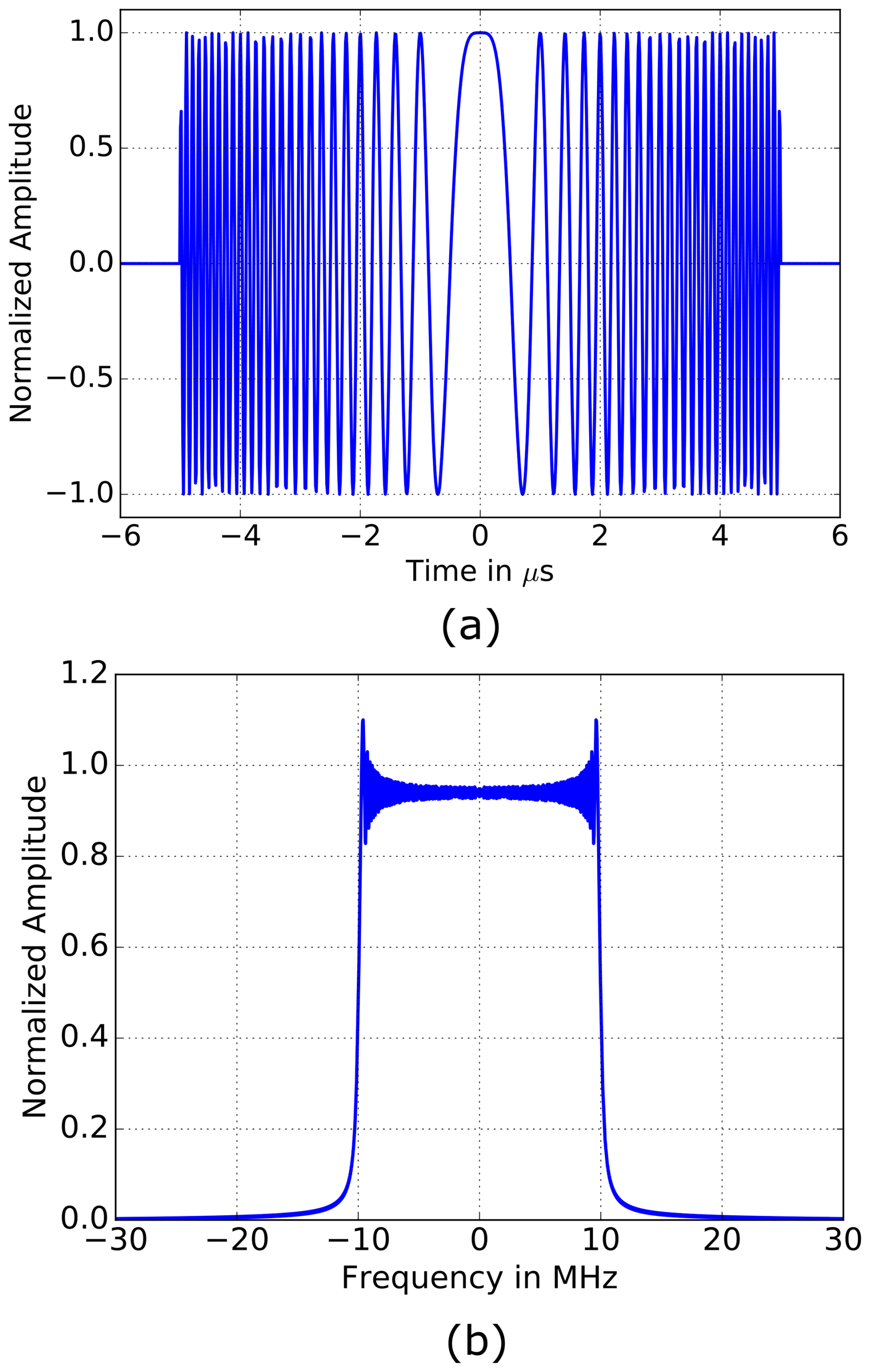
Figure 1 Standard chirp signal in time- and frequency domain with τ_p=10 µs and B=20 MHz. (a) Up-chirp in base-band and time-domain. (b) Up-chirp in base-band and frequency-domain.

It is known that the Fourier transform of the chirp-signal-envelope is not rectangular due to ringing artifacts at the edges of the spectrum. These result from the Fourier series expansion and are known as the Gibbs phenomenon (Gibbs, 1899; Chitode, 2009). In radar, they result in higher sidelobes of the impulse response after range compression. However, in a single-channel system these artifacts can be easily compensated by windowing during the pulse compression process. For multichannel radars, this is not possible because the discontinuities are also located within the waveform spectrum, not just at either end. Therefore, a more detailed analysis is required, which is given in Sect. 5. The Fourier transform of a chirp signal can be expressed as

$$\begin{array}{}\text{(3)}& \begin{array}{rl}{S}_{\mathrm{BB},\text{chirp}}\left(f\right)& =\mathcal{F}\left\{s_{\mathrm{BB},\text{chirp}}\left(t\right)\right\}\\ & ={\displaystyle \frac{\mathrm{1}}{\sqrt{\mathrm{2}\mathit{\pi }}}}\int s_{\mathrm{BB},\text{chirp}}\left(t\right)\cdot \exp \left(-\mathrm{j}\mathrm{2}\mathit{\pi }ft\right)\text{d}t\end{array}\end{array}$$

which is plotted in Fig. 1b for B=20 MHz and τ_p=10 µs.

All of the following suggested MIMO waveforms have this chirp-like structure.

2.2 Orthogonality in SAR and Waveform Separation

The requirements for MIMO radar and MIMO SAR are quite different. In conventional MIMO radar applications, a stringent separation of the waveforms is often not necessary because they are typically used to detect a few point-like targets (Li and Stoica, 2008). When using signal codes, e.g. Barker codes, a part of the energy is smeared over the scene after pulse compression, but this energy does not disappear. In most radar applications to detect specific targets with a sufficiently low false alarm rate, these codes are adequate (Skolnik, 2008). This is because the interference is very small compared to the optimal impulse response, and the interfering energy can be shifted to spatial locations where no targets are present (He et al., 2012). This concept can also be adopted for more advanced coding and multiplexing that achieve orthogonality in the discrete frequency domain (Xia et al., 2015). For SAR, as a typical example of an imaging radar, orthogonality must be achieved with previously known waveforms for each delay and for the imaged scenario consisting of a multitude of point and distributed targets (e.g. rain forests or crop fields). This is because the unwanted, correlating energy from the other waveforms will add up for every single point target in the observed area after coherent combination. Even when using existing orthogonal codes, the interfering energy smears to the positions of other targets and cannot be resolved. The echoes of the different MIMO transmit signals will completely overlap in the channel and it will be impossible to separate them later in the receiver. Therefore, it is desirable to achieve full orthogonality for arbitrary shifts τ between the signals s_k(t) and s_i(t) (Krieger et al., 2012; Krieger, 2014):

$$\begin{array}{}\text{(4)}& \begin{array}{rl}& \int s_k\left(t\right)\cdot s_i^{*}(t-\mathit{\tau })\text{d}t=\mathrm{0}\\ & \forall \mathit{\tau }\in \mathbb{R},k,i\in {\mathbb{N}}_{\mathrm{0}}^{+}\text{ and }k\ne i,\end{array}\end{array}$$

where s_k(t) and s_i(t) denote two arbitrary waveforms. In any case, this condition simply cannot be achieved with waveforms occupying the same frequency band. This is justified by the fact that in direct analogy to the convolution theorem, there is always a correlation between two signals if they share the same spectrum. The only possible solution is to merge several filtering methods, as proposed in Krieger (2014), Li and Stoica (2008) or San Antonio et al. (2007). They claim and prove that filtering not only in the time-frequency domain but also in the spatial/angular domain via beam-forming allows perfect orthogonal conditions.

3 MIMO-SAR Waveforms

This section covers five waveform types that share the common chirp-like structure, but have different properties and signal post-processing strategies.

3.1 Up- and Down-Chirp Waveforms

In the past, the use of alternating or even simultaneous up- and down-chirp signals as a kind of orthogonal waveform has been extensively discussed. This modulation concept was examined in more detail in Mittermayer and Martinez (2003). Limited to a maximum number of only N_Tx=2 transmit channels, this type of waveform does not lead to the desired results even for small observation areas. The reason for this can be seen in the plot of the frequency ramps (Fig. 2). s₀(t) and s₁(t) already intersect in the time-frequency plane for a single point target – at a certain point of time, which inevitably leads to cross-correlation interference. Each additional time shift caused by additional point targets results in even more interference. For a SAR with homogeneous extended targets (e.g. rain forests or deserts), the SNR will tend to zero, as proven in Krieger (2014).

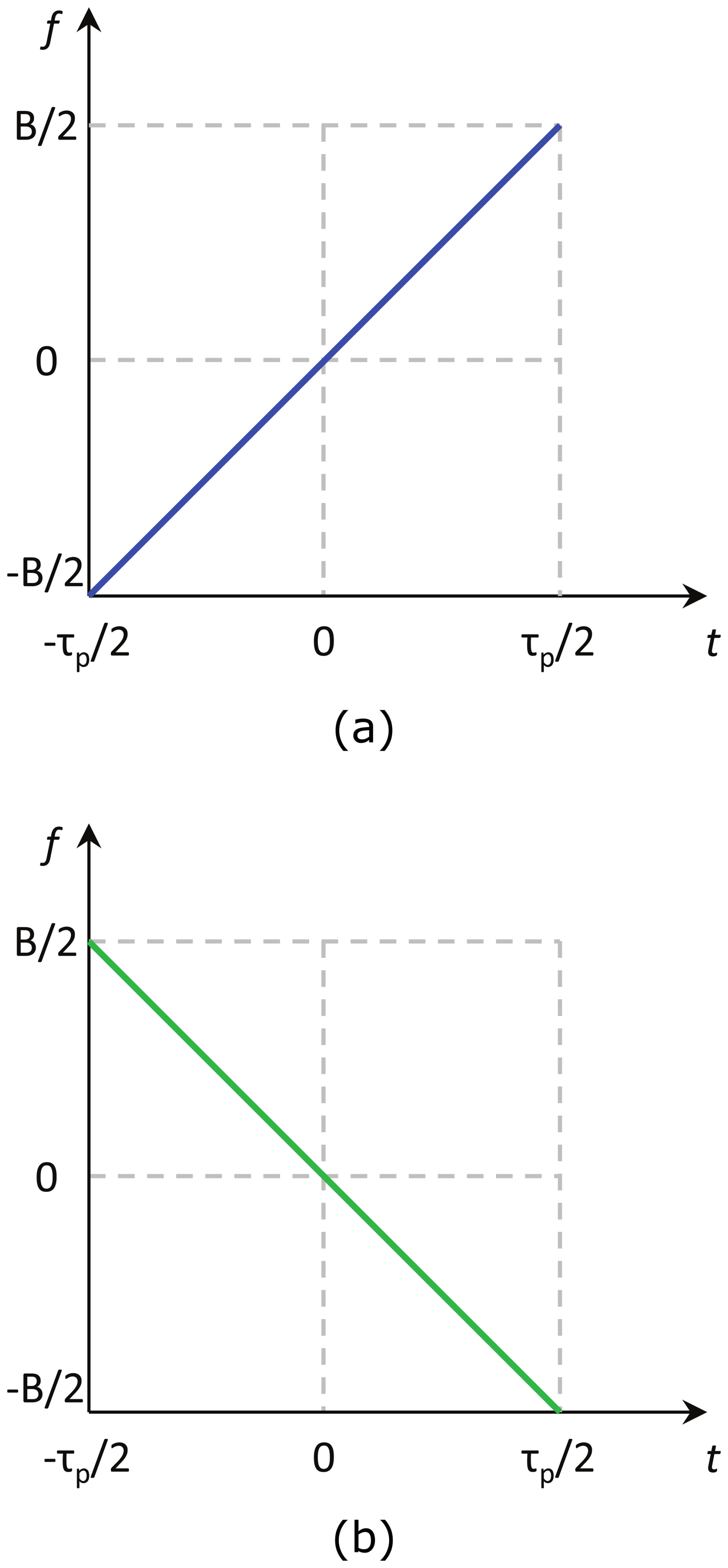
Figure 2 Illustration of the up-down chirp modulation. (a) Signal s₀ (up-chirp). (b) Signal s₁ (down-chirp).

With the recently described knowledge, we will omit this waveform type from further analysis and acknowledge it for completeness.

3.2 OFDM-Chirp Waveforms

OFDM is generally a multicarrier modulation technique. The individual transmit signals occupy the same frequency spectrum, while orthogonality is achieved by periodically interleaving sub-carriers. The OFDM chirp signals were introduced in Kim et al. (2007). In his subsequent publications, this multiplexing technique was further investigated (Kim et al., 2010; Kim, 2011; Kim et al., 2015). Originally defined for two transmit channels only, it is straight forward to extend the scheme to more channels, as will be shown next.

For MIMO-SAR, the OFDM technique is applied to a standard chirp signal, where the total signal duration is τ_p. In contrast to OFDM in communications, where the entire spectrum is occupied at each instance of time, in this context the individual sub-carriers are swept in time due to the chirp-like waveform characteristic. Another difference from classical OFDM is the constant signal envelope with a rectangular shape in the time domain due to the pulse-like character. While a standard chirp occupies the entire frequency spectrum B, the OFDM chirps share it with an interleaved behavior. An example for two transmit signals is shown in Fig. 3. The left side shows the orthogonal sub-carrier scheme for N_Tx=2 and the right side shows the corresponding time-frequency representation. It can be seen that there is a frequency offset of Δf. This so-called sub-carrier offset results in the desired spectral shift of the second waveform to achieve the interleaved carrier structure. Due to the DFT-typical circular time shift property, the suppression of each second discrete frequency sample results in a repetition of the waveform in the time-domain.

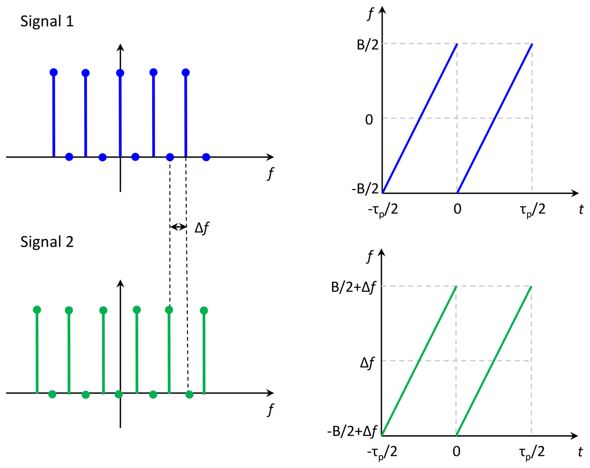
Figure 3 Scheme of the OFDM chirp waveforms for N_Tx=2; left-hand side: signal spectrum; right-hand side: time-frequency relation.

With reference to Eq. (1) an extension of the original definition of the OFDM chirp waveforms from Kim et al. (2007) to an arbitrary number of N_Tx leads to:

$$\begin{array}{}\text{(5)}& \begin{array}{rl}& s_{\mathrm{BB},k}\left(t\right)=\\ & A\cdot \left(\sum _{m=\mathrm{0}}^{N_{\mathrm{Tx}}-\mathrm{1}}\exp \left(\mathrm{j}\mathit{\pi }{K}_{\mathrm{r}}{N}_{\mathrm{Tx}}{\left(t+{\displaystyle \frac{{\mathit{\tau }}_{\mathrm{p}}}{\mathrm{2}}}-{\displaystyle \frac{{\mathit{\tau }}_{\mathrm{p}}(\mathrm{1}+\mathrm{2}m)}{\mathrm{2}{N}_{\mathrm{Tx}}}}\right)}^{\mathrm{2}}\right)\right.\\ & \cdot \left.\mathrm{rect}\left[{\displaystyle \frac{N_{\mathrm{Tx}}(\mathrm{2}t+{\mathit{\tau }}_{\mathrm{p}})-{\mathit{\tau }}_{\mathrm{p}}(\mathrm{1}+\mathrm{2}m)}{\mathrm{2}{\mathit{\tau }}_{\mathrm{p}}}}\right]\right)\cdot \exp \left(\mathrm{j}\mathrm{2}\mathit{\pi }\mathrm{\Delta }fkt\right).\end{array}\end{array}$$

A is the amplitude, which is the same for each transmit waveform and m is the index of the repeated sub-chirp. The last exponential function in Eq. (5) results in the sub-carrier offset of the kth transmit signal. All other terms are equal to the standard chirp except for a shift along the time axis for the signal repetition. The sub-carrier offset Δf depends on the selected number of sub-carriers N_c and the pulse duration τ_p:

$$\begin{array}{}\text{(6)}& \mathrm{\Delta }f={\displaystyle \frac{\mathrm{1}}{N_{\mathrm{c}}{\mathit{\tau }}_{\mathrm{p}}}}.\end{array}$$

N_c is the product of the sampling frequency f_S, which must satisfy the sampling theorem and the signal duration²:

$$\begin{array}{}\text{(7)}& N_{\mathrm{c}}=f_{\mathrm{S}}\cdot {\mathit{\tau }}_{\mathrm{p}}=B\cdot {\mathit{\tau }}_{\mathrm{p}}.\end{array}$$

A plot of a typical MIMO-signal with B=10 MHz, τ_p=10 µs, N_Tx=2 and Δf=1.0 kHz is shown in Fig. 4. For better visualization, the signal has been modulated on a carrier of $f_{\mathrm{0}}=B/\mathrm{2}$. While the repetition of the chirps along the time axis can be seen directly, both waveforms look identical because Δf≪B.

Figure 4 OFDM chirp in time domain with N_Tx=2, τ_p=10 µs, B=10 MHz, Δf=1.0 kHz and $f_{\mathrm{0}}=B/\mathrm{2}$.

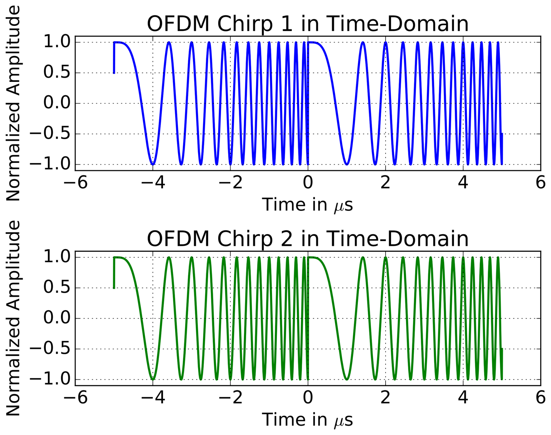
Finally, due to the repetitive structure in the time-domain, the signals are completely orthogonal up to the limit $[-{\mathit{\tau }}_{\mathrm{p}}/N_{\mathrm{Tx}},{\mathit{\tau }}_{\mathrm{p}}/N_{\mathrm{Tx}}]$. If we examine the signals in the frequency domain, orthogonality is only satisfied for frequency shifts less than Δf. This can be explained by the last exponential term in Eq. (5). Irrespective of the number of transmit waveforms, an additional frequency shift of Δf results in $\exp \left(\mathrm{j}\mathrm{2}\mathit{\pi }\mathrm{\Delta }fkt\right)\cdot \exp \left(\mathrm{j}\mathrm{2}\mathit{\pi }\mathrm{\Delta }ft\right)=\exp \left(\mathrm{j}\mathrm{2}\mathit{\pi }\mathrm{\Delta }f(k+\mathrm{1})t\right)$, which is equal to the offset of the next Tx waveform.

It should be noted that OFDM waveform separation in the receiver is complex and computationally intensive. In addition to spatial filtering with Digital Beam-Forming (DBF), it requires techniques to compensate for the orthogonality loss due to the SAR inherent Doppler shift. More details can be found in Kim et al. (2015).

3.3 Multiple Sub-Pulse Mode

The Multiple Sub-Pulse (MSP) mode described in Krieger et al. (2006), Bordoni et al. (2018), Younis et al. (1954) is a mode where multiple chirp-signals of the same length occupying the same frequency band are transmitted (Fig. 5). The individual sub-pulses are transmitted within the same pulse repetition interval and form a single unit. Due to the high time-spread of the propagation channel, the sub-pulses overlap during propagation and must be separated using MIMO-techniques.

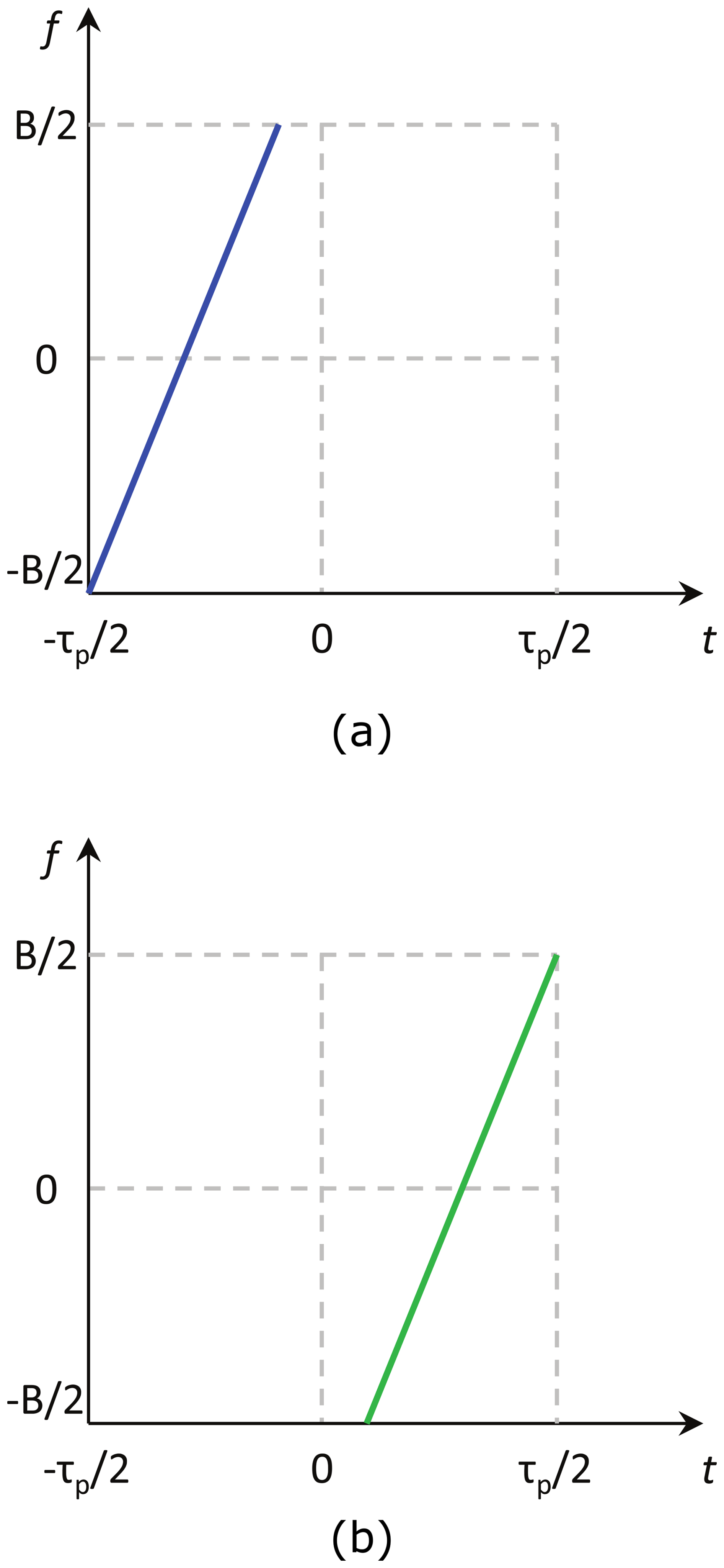
The main changes of a sub-pulse in direct comparison to the single linearly frequency modulated chirp waveform of Eq. (1) are the value of the modulation rate, the reduction of the total pulse duration to τ_sub and a shift on the time-axis to the individual sub-pulse center t_c,k. The common chirp-like characteristic is still preserved. An illustrative MSP signal with the same parameters as for the OFDM chirp signals (B=10 MHz, τ_p=10 µs, N_Tx=2, $f_{\mathrm{0}}=B/\mathrm{2}$) and a gap of τ_s=2 µs is shown in the time-domain in Fig. 5, while Fig. 6 shows the frequency ramps with continuous and equal sweep rate for each sub-pulse.

Figure 5 Illustration of the MSP waveforms with B=10 MHz, τ_p=10 µs, τ_s=2 µs, N_Tx=2, $f_{\mathrm{0}}=B/\mathrm{2}$.

Figure 6 MSP waveform in the time-frequency plane. (a) Signal s₀. (b) Signal s₁.

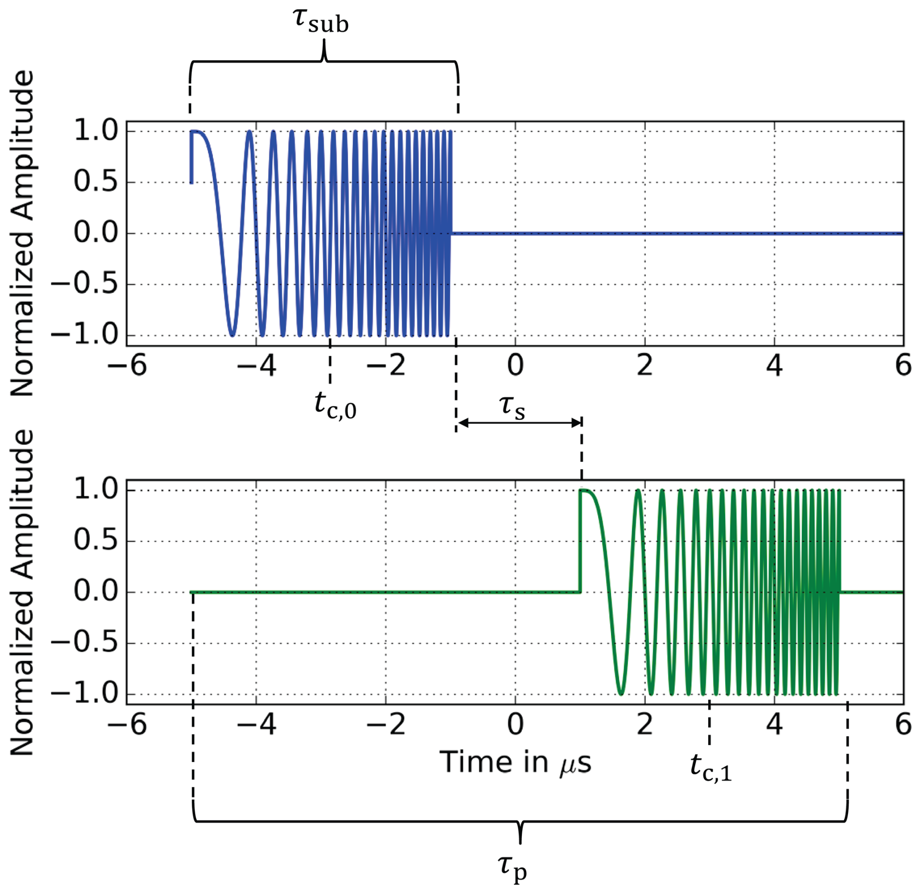
To have a common basis for later waveform comparison, τ_p is set equal for the total signal duration of all signals introduced in this paper. As mentioned before, in the MSP mode, the duration of each sub-pulse is reduced to τ_sub, whith positive or negative gaps of value τ_s between them. The sub-pulse duration, which is the N_Txth fraction of τ_p minus the sum of all gaps is

$$\begin{array}{}\text{(8)}& {\mathit{\tau }}_{\mathrm{sub}}={\displaystyle \frac{{\mathit{\tau }}_{\mathrm{p}}-(N_{\mathrm{Tx}}-\mathrm{1}){\mathit{\tau }}_{\mathrm{s}}}{N_{\mathrm{Tx}}}}.\end{array}$$

Since all sub-pulses have the full signal bandwidth to preserve the range resolution, the chirp must sweep within the shorter time-interval of τ_sub and the modulation rate of Eq. (2) must be redefined to a higher chirp-rate:

$$\begin{array}{}\text{(9)}& K_{\mathrm{r},\mathrm{sub}}=\pm {\displaystyle \frac{B}{{\mathit{\tau }}_{\mathrm{sub}}}}=\pm {\displaystyle \frac{B\cdot N_{\mathrm{Tx}}}{{\mathit{\tau }}_{\mathrm{p}}-(N_{\mathrm{Tx}}-\mathrm{1}){\mathit{\tau }}_{\mathrm{s}}}}.\end{array}$$

For completeness, the shift of the sub-pulses along the time-axis and thus the center of the kth sub-pulse can be expressed by

$$\begin{array}{}\text{(10)}& t_{\mathrm{c},k}=-{\displaystyle \frac{{\mathit{\tau }}_{\mathrm{p}}}{\mathrm{2}}}+{\displaystyle \frac{{\mathit{\tau }}_{\mathrm{sub}}}{\mathrm{2}}}+k{\mathit{\tau }}_{\mathrm{sub}}+k{\mathit{\tau }}_{\mathrm{s}}.\end{array}$$

The final description of the kth sub-pulse reads as follows:

$$\begin{array}{}\text{(11)}& s_{\mathrm{BB},k}\left(t\right)=A\cdot \exp \left(\mathrm{j}\mathit{\pi }{K}_{\mathrm{r},\mathrm{sub}}(t-t_{\mathrm{c},k}{)}^{\mathrm{2}}\right)\cdot \mathrm{rect}\left[{\displaystyle \frac{t-t_{\mathrm{c},k}}{{\mathit{\tau }}_{\mathrm{sub}}}}\right].\end{array}$$

3.4 Segmentally-Shifted Chirp Waveforms

Another promising waveform for MIMO-SAR was proposed in Krieger et al. (2012), later refined in Krieger (2014) and first verified by an experiment in Rommel et al. (2013). In the following we will call it the Segmentally-Shifted Chirp (SSC) waveform. Basically, it consists of shifted chirp waveforms with the same modulation rate but different sub-pulse durations and bandwidths. Each two sub-pulses are combined into a single transmit signal of full bandwidth B and full pulse duration τ_p. To give an example in Fig. 7, the SSC signal is plotted in the time-domain for B=10 MHz, τ_p=10 µs, N_Tx=2 and $f_{\mathrm{0}}=B/\mathrm{2}$. The upper plot shows the first waveform, which consists of segments of the first waveform within τ_p that have been repositioned. In the absence of the first transmit signal, each waveform consists of two sub-pulses, using the full bandwidth and full pulse duration.

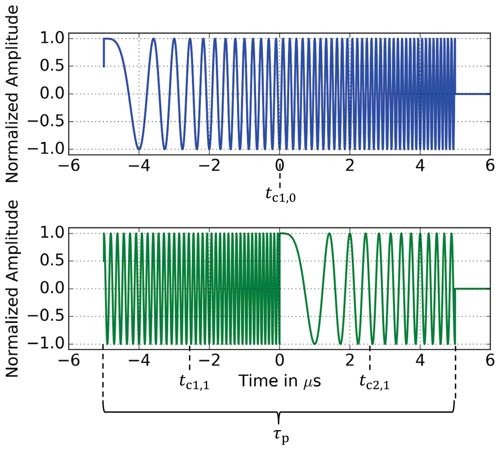
Figure 7 Illustration of the segmentally-shifted chirp waveform in time-domain for B=10 MHz, τ_p=10 µs, N_Tx=2 and $f_{\mathrm{0}}=B/\mathrm{2}$. Upper plot: s₀(t). Lower plot: s₁(t).

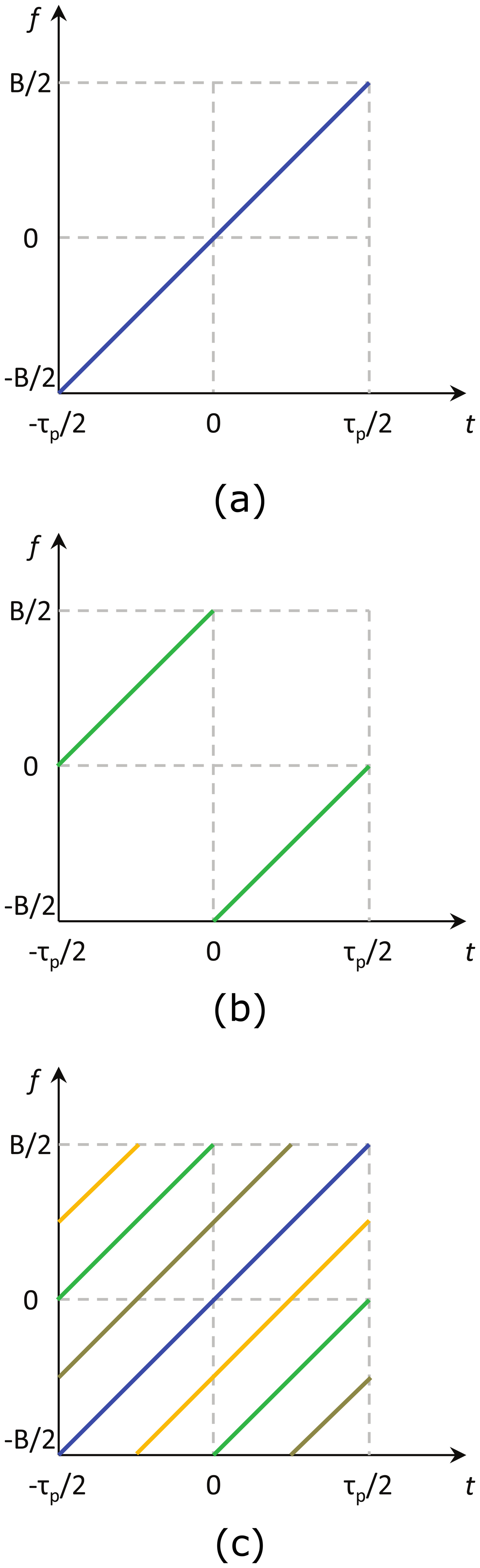
Figure 8 Segmentally-shifted chirp waveform in the time-frequency plane. (a) Signal s_BB,0 for two activated transmit channels. (b) Signal s_BB,1 for two activated transmit channels. (c) Signals s_BB,0 – s_BB,3 for four activated transmit channels.

In order to satisfy the orthogonality condition, the sub-chirps follow a certain sequence, which can be clearly seen in the time-frequency plots in Fig. 8a and b for two and in Fig. 8c for four activated transmit channels. While the modulation rate is the same for each waveform as defined in Eq. (2), we need two sub-pulse centers t_c1,k and t_c2,k for each split sub-pulse. They are defined as

$$\begin{array}{}\text{(12)}& t_{\mathrm{c}\mathrm{1},k}={\displaystyle \frac{k{\mathit{\tau }}_{\mathrm{p}}}{\mathrm{2}{N}_{\mathrm{Tx}}}}\end{array}$$

and

$$\begin{array}{}\text{(13)}& t_{\mathrm{c}\mathrm{2},k}=-{\displaystyle \frac{(N_{\mathrm{Tx}}-k){\mathit{\tau }}_{\mathrm{p}}}{\mathrm{2}{N}_{\mathrm{Tx}}}}.\end{array}$$

The duration of the sub-chirps are

$$\begin{array}{}\text{(14)}& {\mathit{\tau }}_{\mathrm{sub}\mathrm{1},k}={\displaystyle \frac{(N_{\mathrm{Tx}}-k){\mathit{\tau }}_{\mathrm{p}}}{N_{\mathrm{Tx}}}}\end{array}$$

and

$$\begin{array}{}\text{(15)}& {\mathit{\tau }}_{\mathrm{sub}\mathrm{2},k}={\displaystyle \frac{k{\mathit{\tau }}_{\mathrm{p}}}{N_{\mathrm{Tx}}}}.\end{array}$$

It becomes immediately obvious that ${\mathit{\tau }}_{\mathrm{sub}\mathrm{1},k}+{\mathit{\tau }}_{\mathrm{sub}\mathrm{2},k}={\mathit{\tau }}_{\mathrm{p}}$. Using Eqs. (12)–(15) for the standard chirp signal, the SSC waveforms can be written in a closed expression as

$$\begin{array}{}\text{(16)}& \begin{array}{rl}{s}_{\mathrm{BB},k}\left(t\right)& =A\cdot \exp \left(\mathrm{j}\mathit{\pi }{K}_{\mathrm{r}}{\left(t+{\displaystyle \frac{k{\mathit{\tau }}_{\mathrm{p}}}{N_{\mathrm{Tx}}}}\right)}^{\mathrm{2}}\right)\\ & \cdot \exp \left(-\mathrm{j}\mathit{\pi }{\displaystyle \frac{Bk}{N_{\mathrm{Tx}}}}\left(t+{\displaystyle \frac{k{\mathit{\tau }}_{\mathrm{p}}}{N_{\mathrm{Tx}}}}\right)\right)\cdot \mathrm{rect}\left[{\displaystyle \frac{N_{\mathrm{Tx}}t+k{\mathit{\tau }}_{\mathrm{p}}}{(N_{\mathrm{Tx}}-k){\mathit{\tau }}_{\mathrm{p}}}}\right]\\ & +A\cdot \exp \left(\mathrm{j}\mathit{\pi }{K}_{\mathrm{r}}{\left(t-{\displaystyle \frac{(N_{\mathrm{Tx}}-k){\mathit{\tau }}_{\mathrm{p}}}{N_{\mathrm{Tx}}}}\right)}^{\mathrm{2}}\right)\\ & \cdot \exp \left(\mathrm{j}\mathit{\pi }{\displaystyle \frac{B(N_{\mathrm{Tx}}-k)}{N_{\mathrm{Tx}}}}\left(t-{\displaystyle \frac{(N_{\mathrm{Tx}}-k){\mathit{\tau }}_{\mathrm{p}}}{N_{\mathrm{Tx}}}}\right)\right)\\ & \cdot \mathrm{rect}\left[{\displaystyle \frac{N_{\mathrm{Tx}}t-(N_{\mathrm{Tx}}-k){\mathit{\tau }}_{\mathrm{p}}}{k{\mathit{\tau }}_{\mathrm{p}}}}\right]\text{ for }k>\mathrm{0}.\end{array}\end{array}$$

For k=0 Eq. (1) must be taken, since the first transmit waveform is the standard chirp waveform, with full bandwidth and full pulse duration.

3.5 Chirp Diverse Waveforms

The chirp diverse waveforms were proposed by Wang and published in Wang (2011), Wang and Cai (2012), Wang (2015). In this OFDM-based technique, multiple short sub-pulses are generated and modulated on individual sub-carriers. The number of carriers is smaller than in classical OFDM signals, but usually larger than the number of transmit channels. Furthermore, the number of simultaneously active sub-carriers is independent of the number of sub-pulses, and up- and down-chirp modulation can be used in parallel. As suggested in Wang (2015), a random matrix modulation concept helps to optimize the auto- and cross-correlation interference between the waveforms. A set of many short sub-chirp signals shifted in the time-frequency plane is generated. An example with N_Tx=2 is shown in the time-frequency plane in Fig. 9.

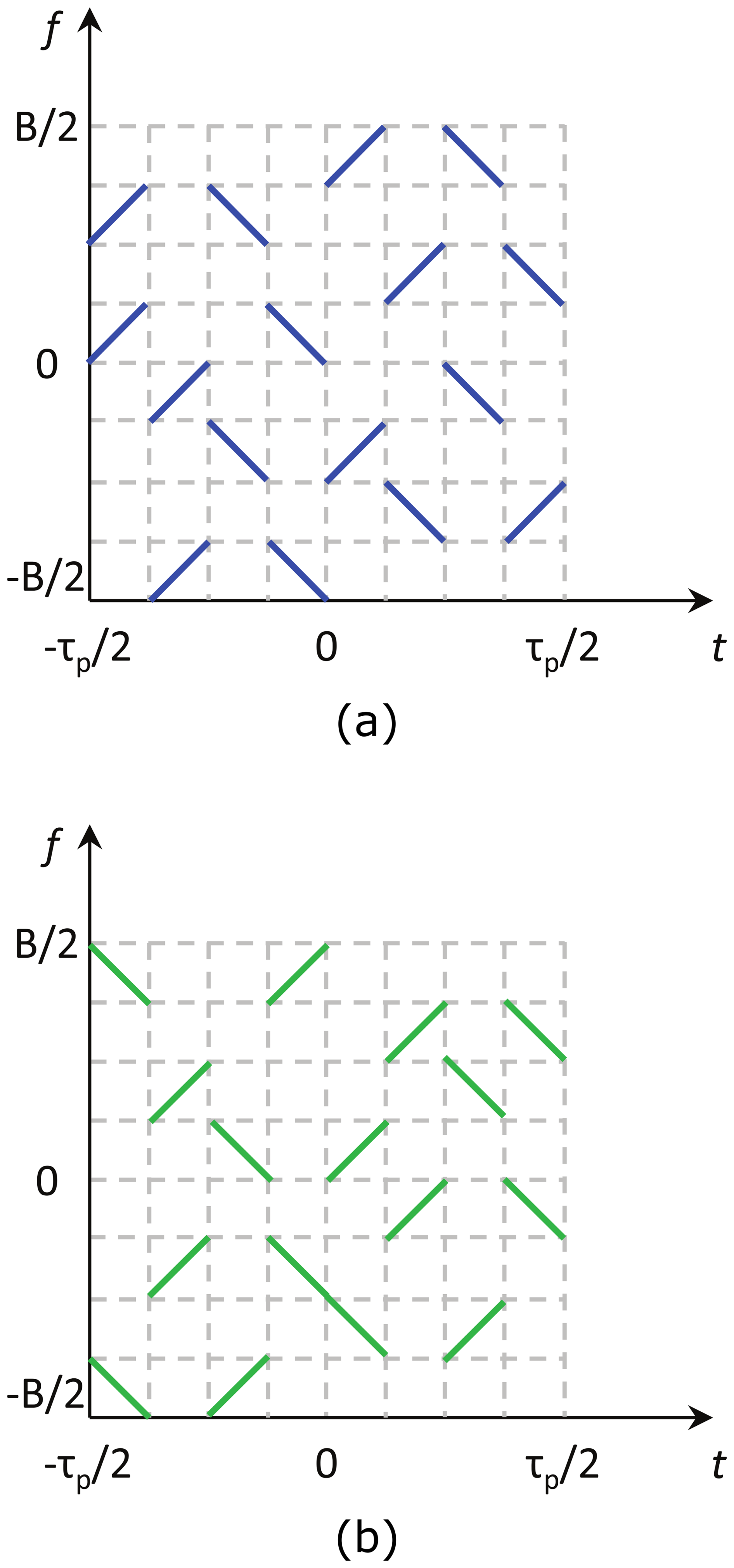
Figure 9 Illustration of the chirp diverse waveforms with N_Tx=2 in the time-frequency plane. (a) Chirp diverse signal s₀. (b) Chirp diverse signal s₁.

Simulation results with narrow swath widths show in Wang (2015) that this waveform type is promising for MIMO-SAR. However, it was shown in Krieger (2014), that this multiplex concept does not work for distributed scenarios with millions of scatterers. As it can be seen from the time-frequency plots in Fig. 9, even small time shifts of s₀ and s₁ lead to overlapping of sub-chirps and thus to cross-correlation interference.

4 Ambiguity Function

To analyze the behavior of a radar waveform in terms of resolution, cross- and auto-correlation interference and Doppler tolerance, it has been found that the Ambiguity Function (AF) is an important tool. There are now a number of AFs, each focusing on different effects, while most functions are based on the first AF defined by Woodward in 1967 (Woodward, 1967). Besides Woodward's AF, the most important AFs are the SAR Ambiguity Function defined by Harger in 1965 (Harger, 1965), the MIMO radar AF defined by San Antonio et al. (2007) and the Transmit Beamspace AF of Li et al. (2015). Since the SAR-AF is not primarily a function of the radar waveforms, it shows dependencies on antenna characteristics, ISLR and azimuth resolution. In particular, it analyzes the azimuth and range ambiguities. In order to focus on the waveforms themselves, a special case of the MIMO radar AF and the Transmit Beamspace AF is considered in this section.

4.1 Description of the Ambiguity Function

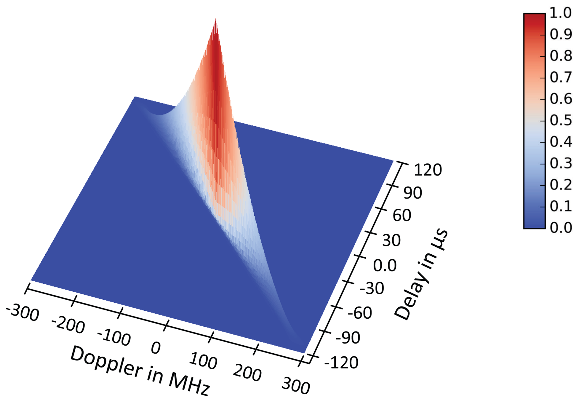
First, we focus on a single waveform with optimal characteristics for radar. The basic auto-correlation of a single waveform can then be represented graphically using Woodward's AF (Woodward, 1967). The ambiguity function of the kth waveform is defined as the squared magnitude of

$$\begin{array}{}\text{(17)}& {\mathit{\chi }}_k(\mathit{\tau },f_{\mathit{\nu }})=\int s_k\left(t\right)\cdot s_k^{*}(t-\mathit{\tau })e^{\mathrm{j}\mathrm{2}\mathit{\pi }{f}_{\mathit{\nu }}t}\text{d}t.\end{array}$$

It basically reflects the normalized matched filter at different combinations of range delays τ and Doppler shifts f_ν. In the typical 3D surface plot representation of the AF, these two parameters correspond to the axes, while the magnitude is given by ${\left|{\mathit{\chi }}_k\right|}^{\mathrm{2}}$. This gives an idea of how the radar system responds to targets at different ranges and velocities. For a standard radar chirp signal with B = 300 MHz and a pulse duration of τ_p = 120 µs, the ridge in the ambiguity function of Fig. 10 represents the area of maximum response. The width and shape of the ridge provide insight into the resolution of the radar in both the range and velocity domains, with a narrower ridge indicating better resolution. More specifically, the AF plot in the center at f_ν=0 Hz along the τ axis shows the impulse response of the waveform with its 3 dB width as range resolution.

Figure 10 Woodward's Ambiguity Function of an up-chirp with B=300 MHz and τ_p=120 µs.

In recent years, a number of MIMO radar Ambiguity Functions have been derived. They focus on different properties of the radar and are therefore not directly comparable. In 2007, San Antonio et al. (2007) developed a very good evaluation of these functions and introduced a generalized MIMO AF, which was later further analyzed by Chen (Chen and Vaidyanathan, 2008). San Antonio showed that the MIMO Ambiguity Function depends not only on the signal itself, but also on the radar system, the beam-forming algorithm used, and the target. Basically, the MIMO AF shows that the unwanted correlated signal energy can also be suppressed by proper beam-forming. This equation takes into account all the parameters of the radar system, including the element spacing, the antenna beam patterns, the channel characteristics and the backscattering characteristics of the targets. The function presented in San Antonio et al. (2007) depends on 16 independent parameters.

Because several factors are involved, an analytical solution of this function is not readily possible. For this reason, Chen defined in Chen and Vaidyanathan (2008) a simplified form, also known as the Cross Ambiguity Function, which focuses on the fundamental correlation between multiple transmit waveforms. For the derivation, Chen introduced constraints that are valid for most MIMO radar systems:

• No analog beam-forming/no analog spatial filtering

• Targets are localized in the far field

• High time-bandwidth product: TB>100

• Collocated antenna array – no bistatic/multistatic geometrical description

• Narrow-band assumption: $B/\mathrm{2}<f_{\mathrm{0}}$.

The Cross AF reads as follows:

$$\begin{array}{}\text{(18)}& \begin{array}{rl}& {\mathit{\chi }}_k^{\prime }(\mathit{\tau },f_{\mathit{\nu }})=\int s_k\left(t\right)\cdot \left[s_k^{*}(t-\mathit{\tau })+\sum _b{s}_b^{*}(t-\mathit{\tau })\right]e^{\mathrm{j}\mathrm{2}\mathit{\pi }{f}_{\mathit{\nu }}t}\text{d}t\\ & \text{for }b\in {\mathbb{N}}_{\mathrm{0}}^{+},b<N_{\mathrm{Tx}}\text{ and }b\ne k.\end{array}\end{array}$$

Since the correlation is a linear operation, it is reasonable to split Eq. (18) up into two parts:

$$\begin{array}{}\text{(19)}& \begin{array}{rl}{\mathit{\chi }}_k^{\prime }(\mathit{\tau },f_{\mathit{\nu }})& =\int s_k\left(t\right)\cdot s_k^{*}(t-\mathit{\tau })e^{\mathrm{j}\mathrm{2}\mathit{\pi }{f}_{\mathit{\nu }}t}\text{d}t\\ & +\int s_k\left(t\right)\cdot \sum _b{s}_b^{*}(t-\mathit{\tau })e^{\mathrm{j}\mathrm{2}\mathit{\pi }{f}_{\mathit{\nu }}t}\text{d}t\\ & ={\mathit{\chi }}_k(\mathit{\tau },f_{\mathit{\nu }})+{\mathit{\varsigma }}_k(\mathit{\tau },f_{\mathit{\nu }}),\end{array}\end{array}$$

with

$$\begin{array}{}\text{(20)}& {\mathit{\varsigma }}_k(\mathit{\tau },f_{\mathit{\nu }})=\int s_k\left(t\right)\cdot \sum _b{s}_b^{*}(t-\mathit{\tau })e^{\mathrm{j}\mathrm{2}\mathit{\pi }{f}_{\mathit{\nu }}t}\text{d}t.\end{array}$$

The first additive part of Eq. (19) is equal to the function defined by Woodward in Eq. (17), while the second part Eq. (20) describes the unwanted interference with the other transmitted waveforms. A signal suitable for MIMO-SAR should have a χ_k as shown in Fig. 10, while ς_k,b should ideally be zero for all time and frequency shifts. Alternatively, the interference in ς_k can be removed by analogue beam-forming or DBF in a separate post-processing step.

A major difference between the MIMO AF and the Transmit Beamspace AF (Li et al., 2015) is that the TB-AF is more general and also deals with coherent transmit signals, which are not the topic of this paper and therefore are not mentioned in the further analysis.

4.2 Ambiguity Function Analysis

Figure 11 shows the plots of the Cross Ambiguity Functions for the OFDM chirp signals, the MSP mode, the SSC waveforms and for the Chirp Diverse waveforms for N_Tx=2. Each set of waveforms has a total bandwidth of 300 MHz and a total pulse duration of 120 µs. An important extraction from the three-dimensional AF plots are the zero-Doppler cuts, which express the impulse response for a point target in a static scene (f_ν=0 Hz). They can be found on the right side of Fig. 11. It can be clearly seen that the desired (main-lobe) in the center has exactly the same shape as for a standard up-chirp, except for the Chirp Diverse waveforms. The ambiguities resulting from cross-correlation with the second transmit waveform are concentrated on dedicated, localized ridges for the three waveform types. This allows removal of this unwanted energy by time-varying beam-forming in post-processing. The AF of the Chirp Diverse waveform shows pronounced interference that is randomly distributed throughout the entire time-frequency plane.

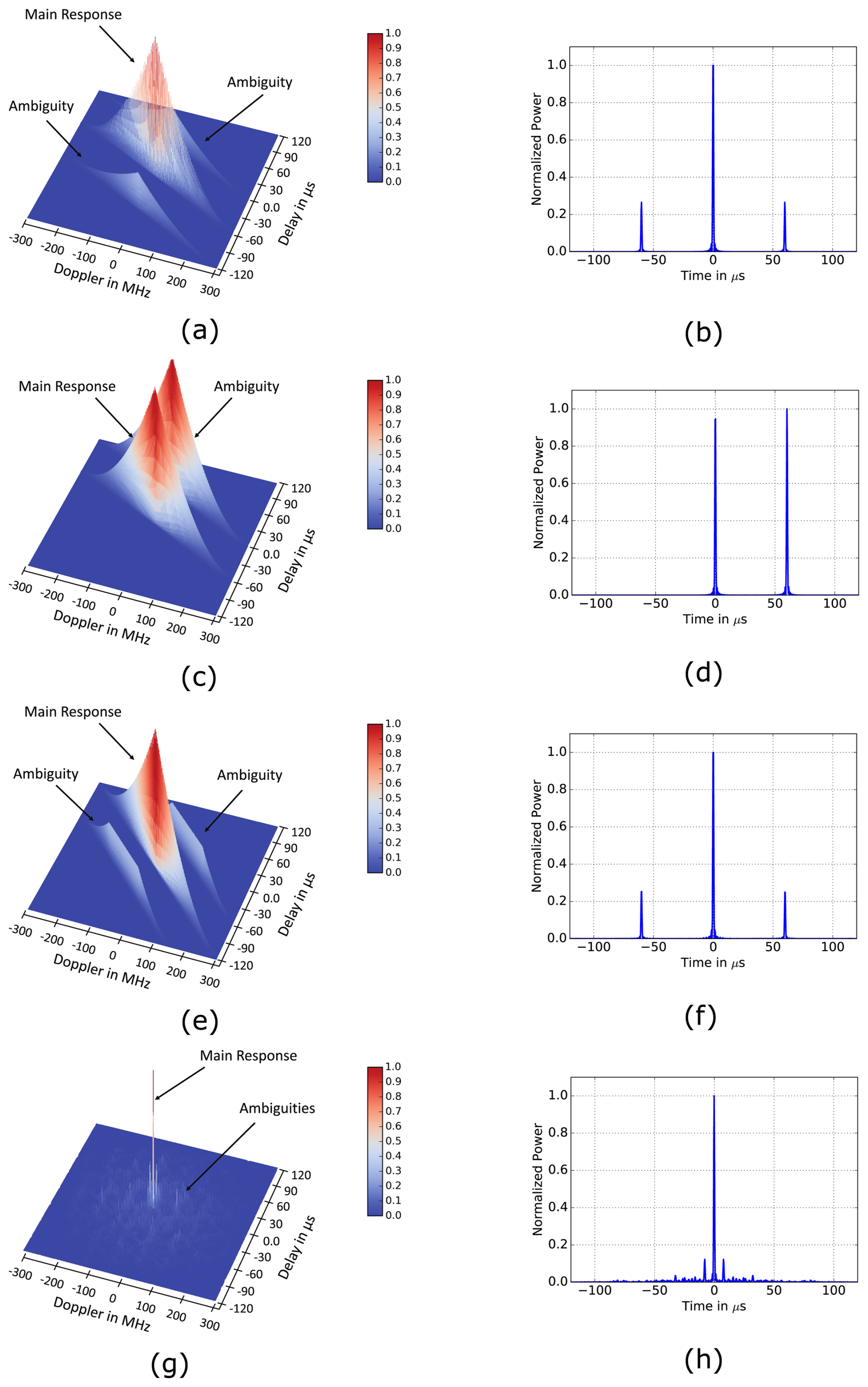
Figure 11 Cross-Ambiguity Functions with corresponding zero-Doppler cuts (Eq. 19) of different waveforms. (a) Cross-AF of OFDM chirp signal. (b) $\left|{\mathit{\chi }}^{\prime }\right(\mathit{\tau },\mathrm{0}){|}^{\mathrm{2}}$ of OFDM chirp signal. (c) Cross-AF of MSP mode. (d) $\left|{\mathit{\chi }}^{\prime }\right(\mathit{\tau },\mathrm{0}){|}^{\mathrm{2}}$ of MSP mode. (e) Cross-AF of SSC waveform. (f) $\left|{\mathit{\chi }}^{\prime }\right(\mathit{\tau },\mathrm{0}){|}^{\mathrm{2}}$ of SSC waveform. (g) Cross-AF of Chirp Diverse waveform. (h) ${\mathit{\chi }}^{\prime }(\mathit{\tau },\mathrm{0}){|}^{\mathrm{2}}$ of Chirp Diverse waveform.

A noticeable artifact in the OFDM AF plot is that the ridge in the center is not completely filled due to the interleaving behavior of the sub-carriers. The repetitive structure of each OFDM chirp also introduces auto-correlation interference, which are superimposed on the cross-correlation interference. However, due to the sub-carrier spacing, the waveforms can be separated. Since only half of the full waveform is correlated at each each ambiguous ridge, only half of the signal energy is focused on such an ambiguity. In addition, each of the repeated sub-pulses implies the full signal bandwidth. The width of the ridge, and therefore the resolution, is also the same.

Basically, the MSP mode is just a sequence of repeated chirp waveforms. As a result, the signal ambiguities have the same energy and resolution as the main impulse response. The result is an exact replication of the main impulse response.

With the exception of the first waveform, all other waveforms in the SSC waveform mode consist of two shifted sub-pulses. This results in two ambiguities for each subsequent transmitted signal. Each ambiguity shares half of the signal energy and half of the total bandwidth. This means that the signal ambiguities to be suppressed have half the amplitude and half the resolution of the auto-correlation. It is worth noting that in the later application, due to the projection of the signal onto the spherical Earth ground, the positions of the signal ambiguities are not symmetrical, leading to a more complicated pattern synthesis for DBF suppression.

Because the Chirp Diverse waveform typically consists of several short sub-chirps with overlapping spectra, certain sub-pulses will correlate at certain time or frequency shifts. This is also the case for a single transmit waveform. Accordingly, the energy of both waveforms is smeared in the AF plot. This fact alone makes this waveform type inapplicable for MIMO-SAR.

An advantage of the OFDM, MSP and SSC waveforms is that they all have the same requirements for additional filtering because the separation between the signal ambiguities and the main response is the same. As already mentioned by San Antonio et al. (2007) and Krieger et al. (2006), the energy in the auto- and cross-correlation interferences can be suppressed by DBF. Using a priori knowledge of the scene geometry, antennas and waveforms, appropriate antenna patterns can be synthesized during post-processing to enable MIMO-SAR without interference from the radar's own waveforms.

5 Waveform Performance Parameters

This section summarizes a list of the most important decision parameters in radar waveform analysis. It can be used to rank future MIMO radar waveforms in their performance in terms of resolution, energy budget, interference and practicality. Using a decision matrix, the radar designer can easily select the most appropriate signal for the application.

5.1 Range Resolution

By definition, resolution is the ability to detect two identical objects separated by a minimum distance δ_rg and to resolve them from each other (IEEE Standard Radar Definitions, 1998). The range resolution is along the radial direction from the radar, while the azimuth and elevation angles are constant. To separate the backscattered signals from these two targets, it is mandatory to separate at least the two leading edges of the pulses from each other, since the radar signals are usually modulated (also called intrapulse modulation). The maximum achievable range resolution of a radar is defined as (Skolnik, 2008)

$$\begin{array}{}\text{(21)}& {\mathit{\delta }}_{\mathrm{rg}}=w_{\mathrm{win}}\cdot {\displaystyle \frac{c}{\mathrm{2}B}},\end{array}$$

where w_win is a scalar, characteristic value for the window function used during the range compression process. Common values are w_win=0.886 for a rectangular window and w_win=1.3 for a Hann window (Cumming and Wong, 2005). This maximum resolution can only be achieved if the transmit signal envelope is perfectly rectangular, which is the case for all four proposed waveform types (OFDM, MSP, SSC, and Chirp Diverse waveforms). In all other cases, any variations in the pulse shape will result in reduced resolution.

Instead of using Eq. (21), it is also possible to determine the resolution from the 3 dB-width of the impulse response, which corresponds to the centered sinc-function in the zero-Doppler cuts of the AF (Fig. 11). Both methods give the same result. Simulations for different numbers of Tx waveforms N_Tx have shown that each of the previously defined waveforms shares the full bandwidth and therefore has the same resolution characteristics.

5.2 Integrated Sidelobe Ratio

In this subsection, we analyze the effects on the Integrated Sidelobe Ratio (ISLR). By definition, the ISLR is an indicator of the amount of energy in the sidelobes of the impulse response relative to the amount of energy in the main-lobe of the impulse response (Cumming and Wong, 2005). Thus, a low ISLR is preferred. In Fig. 12 both amounts of energy are marked in green and blue, respectively. Typically, the energy in the side-lobes is not fully accounted for. While the impulse response function has a total width of τ_p after pulse compression, the ISLR uses only the time segment ΔT. Following the definition of the ISLR (Cumming and Wong, 2005), for a given observation time ΔT we get:

$$\begin{array}{}\text{(22)}& \begin{array}{rl}& \text{ISLR}\left(\mathrm{\Delta }T\right)={\displaystyle \frac{\underset{-\mathrm{\Delta }T/\mathrm{2}}{\overset{-T_{\mathrm{NBW}}/\mathrm{2}}{\int }}{\mathit{\chi }}_k^{\prime }(\mathit{\tau },\mathrm{0})\text{d}\mathit{\tau }+\underset{T_{\mathrm{NBW}}/\mathrm{2}}{\overset{\mathrm{\Delta }T/\mathrm{2}}{\int }}{\mathit{\chi }}_k^{\prime }(\mathit{\tau },\mathrm{0})\text{d}\mathit{\tau }}{\underset{-T_{\mathrm{NBW}}/\mathrm{2}}{\overset{T_{\mathrm{NBW}}/\mathrm{2}}{\int }}{\mathit{\chi }}_k^{\prime }(\mathit{\tau },\mathrm{0})\text{d}\mathit{\tau }}}\\ & \forall T_{\mathrm{NBW}}\le \mathrm{\Delta }T\le {\mathit{\tau }}_{\mathrm{p}},\end{array}\end{array}$$

where T_NBW is the null-to-null-beamwidth and approximately twice the 3dB-width of the impulse response.

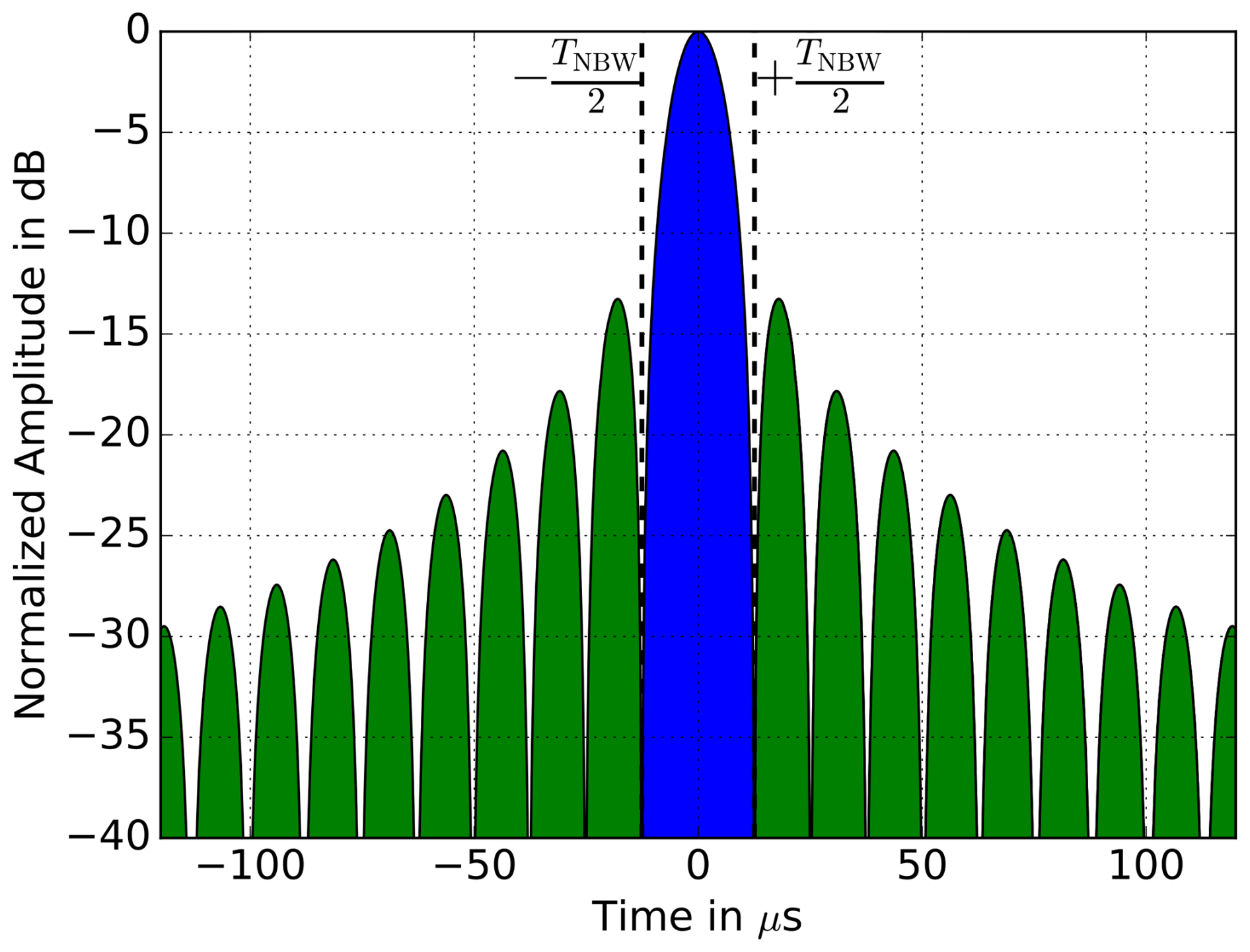
Figure 12 Impulse response function of a linearly frequency modulated chirp signal. The green surface indicated the amount of energy within the sidelobes and the blue surface the energy within the main-lobe. The ratio between the two is defined as ISLR.

A typical value for the impulse response of a chirp signal is ISLR = −9.8 dB. The RCS of different targets within a standard SAR scene will usually exceed this value, and sidelobes from a strong scatterer can blur the rest of the image. Therefore, it is recommended to apply windowing to overcome the steep slopes at the edges of the chirp spectrum. For example, Hann windowing can significantly reduce the ISLR to about −21 dB, while degrading the resolution by a factor of w_win (see Eq. 21). Windowing affects the ISLR mainly for small values of ΔT. Especially for MIMO-waveforms, where ambiguities naturally occur, for larger ΔT ($\mathrm{\Delta }T>{\mathit{\tau }}_{\mathrm{p}}/N_{\mathrm{Tx}}$) the cross- and auto-correlation interferences lead to significant contributions to the ISLR. Since they are typically suppressed by DBF and null-steering techniques during post-processing, analyzing the full range of ΔT is mainly useful to study the waveforms, but not for a fair comparison.

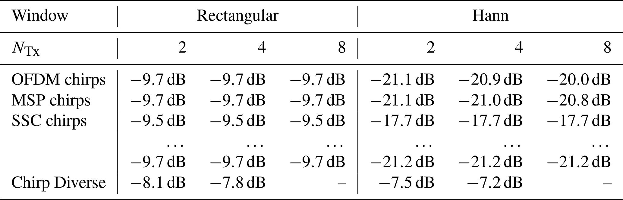
For a meaningful analysis, the ISLR was calculated for different values of ΔT, N_Tx and window types. To have a common base, the following simulation parameters were used: B=300 MHz, τ_p=120 µs and N_Tx=4. The results can be found in Fig. 13 and Table 1 and general observations can be made. Across all plots in Fig. 13, the ISLR increases in a stepwise manner. As indicated by the zero-Doppler cuts of the AF, observation times outside the interval $\left[-\frac{{\mathit{\tau }}_{\mathrm{p}}}{N_{\mathrm{Tx}}},\frac{{\mathit{\tau }}_{\mathrm{p}}}{N_{\mathrm{Tx}}}\right]$ produce strong ambiguities, which cause the ISLR value jumps shown in Fig. 13. For sure, after the first step at ${\mathit{\tau }}_{\mathrm{p}}/N_{\mathrm{Tx}}$ the ISLR must always be higher than 0 dB, because not only the full energy of the second transmit waveform applies, but also the energy of the side-lobes of all remaining signals.

5.2.1 OFDM Waveforms

The ISLR can also be seen as an extraction of the zero-Doppler cut, which is plotted on the right side of each ISLR-plot for better comparison (see Fig. 13). The expectations regarding the step-wise increase of the ISLR are fully met. Especially for the OFDM signals, it can be observed that for large ΔT – in direct comparison to the other waveforms – the ISLR improves slightly due to the sub-carrier spacing Δf: They do not fully correlate between the waveforms at the zero-Doppler cut.

Table 1 shows that the ISLR for $\mathrm{\Delta }T<\mathrm{0.1}\cdot {\mathit{\tau }}_{\mathrm{p}}$ is more or less independent of the number of transmit signals. The small degradation for increasing N_Tx with Hann windowing is also an effect of the sub-carrier spacing.

Table 1 Maximum ISLR for small observation intervals ($\mathrm{\Delta }T<\mathrm{0.1}\cdot {\mathit{\tau }}_{\mathrm{p}}$) in dependence on N_Tx, window type and waveform.

5.2.2 MSP Waveforms

Referring to Fig. 11, each additional transmit signal is fully correlated by integer multiples of ${\mathit{\tau }}_{\mathrm{p}}/N_{\mathrm{Tx}}$. After the first ISLR step, where the second sub-pulse correlates, the ISLR increases by 3 dB after each step. For small values of ΔT ($\ll {\mathit{\tau }}_{\mathrm{p}}/N_{\mathrm{Tx}}$) the ISLR shows the same behavior as for the OFDM chirps.

In Table 1, a significant advantage of the MSP mode can be seen: Since the waveforms are just repetitions of the same standard chirp signals, each sub-pulse can be windowed individually because there is no intermodulation transition within a single transmitted sub-pulse waveform. The ISLR will have the same value as for a single linearly frequency modulated chirp. However, as the number of N_Tx increases, the ISLR also decreases (visibly more so for a Hann window). With a larger number of transmit channels, more energy is concentrated at the peaks, but there is also a significant amount within the side-lobes of the impulse response that sums up. Obviously, the higher amount of energy in these sidelobes also affects the ISLR for small ΔT.

5.2.3 SSC Waveforms

The ISLR-plot of the SSC waveforms shows that the behavior is very similar to that of the OFDM signals. However, a major difference is the absence of interleaved sub-carriers, which leads to a higher ISLR for observation times $>(N_{\mathrm{Tx}}-\mathrm{1}){\mathit{\tau }}_{\mathrm{p}}/N_{\mathrm{Tx}}$. The ISLR at these positions is the same as for the MSP mode. Remember that the structure of the SSC waveforms always has an intersection in the signal spectrum due to the sub-pulse transition (cf. Fig. 7), and thus a total of three jump discontinuities. Depending on the position of the intersection, which in turn depends on the channel index k and the total number of transmit channels, the discontinuity can be more or less suppressed by windowing. In the worst case, the discontinuity is centered in the middle of the spectrum (e.g., N_Tx=2, k=1), because there is always the maximum of the windowing function and no suppression occurs. To reduce the discontinuity in the center, it is suggested to smooth the transition between the start and end of the second waveform with a constant phase offset. This can be explained by the fact that this discontinuity is caused by a step function at the intersection of the two sub-chirps in the time-domain.

A closer look at the third row in Table 1 shows that no specific values can be given, since the ISLR depends on k. The best achievable values are the same as for a standard chirp, because the SSC waveform with index k=0 is equal to it. As mentioned before, the minimum ISLR corresponds to the index k=1.

5.2.4 Chirp Diverse Waveforms

The Chirp Diverse waveforms show auto- and cross-correlation interference in the impulse response plot of Fig. 13h. These are not only concentrated at certain positions, but are also smeared along the entire time axis. This is due to the underlying structure of this waveform type with many short sub-chirps that interfere. In particular, high peaks in the plot with a separation of ${\mathit{\tau }}_{\mathrm{p}}/\mathrm{8}$ are an artifact of the sub-chirps that coincide at certain time shifts and are fully correlated³. For short observation intervals ($\mathrm{\Delta }T<{\mathit{\tau }}_{\mathrm{p}}/N_{\mathrm{Tx}}$) the ISLR rises rapidly due to the large amount of interfering energy over the entire extension of the impulse response. The step jumps can be explained by the peaks in the impulse response in Fig. 13h.

In general, this waveform type has a poor ISLR compared to the other three waveform types – even for short observation intervals (see also Table 1). Because four transmit waveforms already fill the entire available structure of the used time-frequency domain grid (Fig. 13h), an extension to N_Tx=8 is not possible.

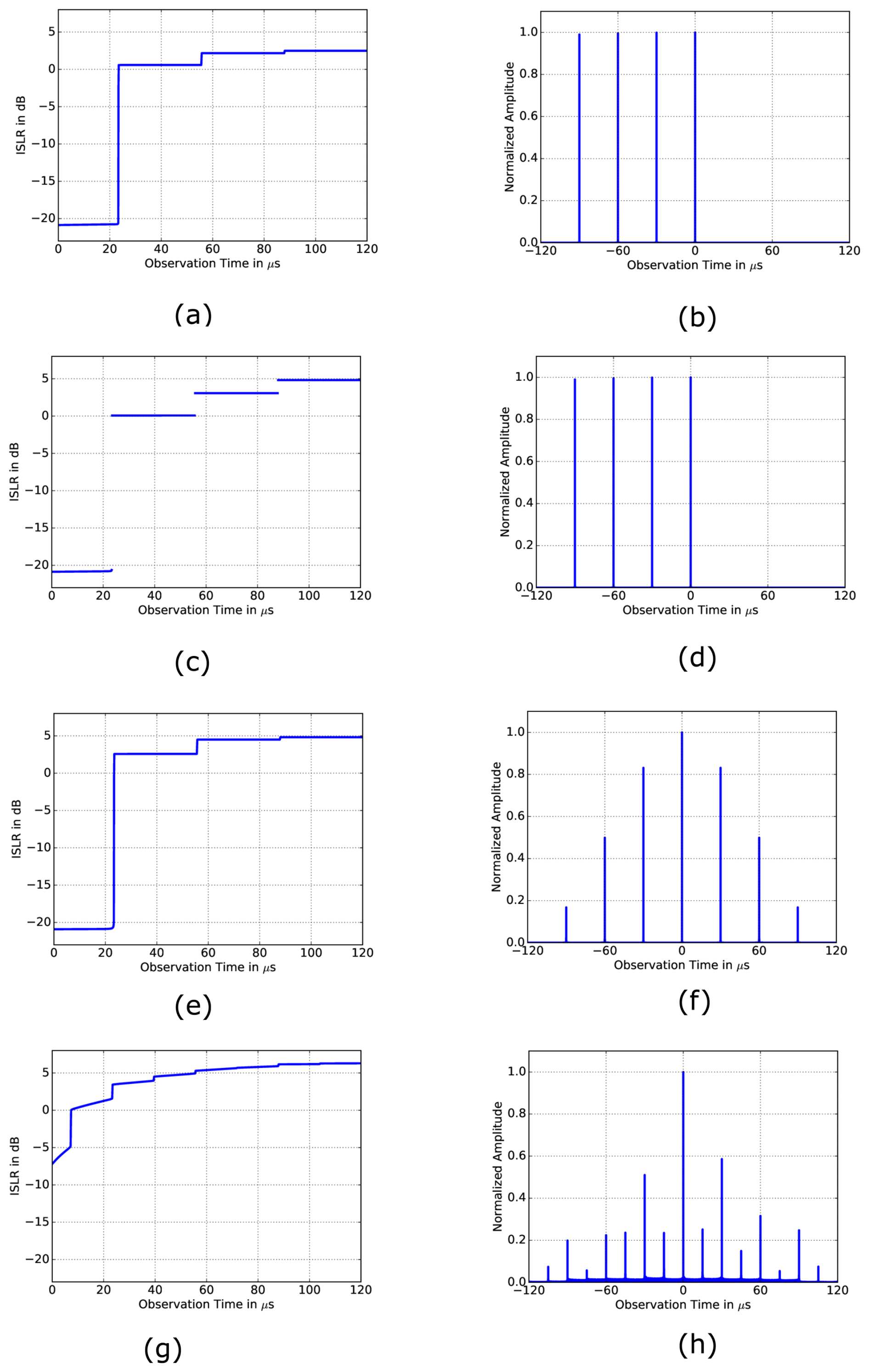
Figure 13 Integrated sidelobe ratios (Eq. 22) with corresponding impulse responses of different waveforms with B=300 MHz, τ_p=120 µs, N_Tx=4 and Hann windowing. (a) ISLR OFDM waveform. (b) Impulse response OFDM waveform. (c) ISLR MSP waveform. (d) Impulse response MSP waveform. (e) ISLR SSC waveform. (f) Impulse response SSC waveform. (g) ISLR Chirp Diverse waveform. (h) Impulse response Chirp Diverse waveform.

5.2.5 Summary of the ISLR Analysis

The ISLR characteristics are comparable between the OFDM and MSP chirps and can compete with those of a single linearly frequency modulated chirp. In particular, the OFDM chirps show better results for a large number of transmit channels due to less cross-correlation interference caused by the sub-carrier spacing. The disadvantage of SSC chirps is that they can lead to pronounced sidelobes in the SAR image if no prior phase correction is applied. The Chirp Diverse waveforms show the worst ISLR of all. At this point, it should be noted that the ideal filter approach (Moreira and Misra, 1995) could be used as an alternative to the standard range compression. This signal compression method achieves optimal results in terms of ISLR for slightly distorted chirp-like signals at a small cost in resolution and signal-to-noise ratio. However, the ideal filter approach would need to be adapted to a time-variant filter in order to cope with the time-variant characteristics of the ambiguities to be removed. This alternative to improve the poor performance of the Chirp Diverse waveforms remains a subject for future research.

5.3 Transmit Energy

The maximum available energy is mainly limited by the instrument resources, the duty cycle, and the gain and efficiency of the amplifier used in the transmitter. The energy of a signal s_k(t) is defined as:

$$\begin{array}{}\text{(23)}& E_k=\underset{-\mathrm{\infty }}{\overset{\mathrm{\infty }}{\int }}\left|s_k\right(t){|}^{\mathrm{2}}\text{d}t,\end{array}$$

which in turn is the auto-correlation (zero lag) of the transmit signal function. In particular, for the signal types mentioned above, the energy is independent of the waveform index k, because in a set of waveforms s(t), each chirp has the same pulse duration. To have a common basis for later illustrative case studies, we define that the total transmit signal energy and the pulse duration τ_p are the same for each waveform type. Consequently, the signal amplitude must be changed for each case.

Beyond the waveform perspective, system-level aspects must also be considered. In general, the available antenna aperture in MIMO-SAR configurations, especially those employing spatial multiplexing, is typically divided among the transmit sub-apertures (N_Tx channels). This reduces the effective radiated energy per channel compared to an equivalent SISO or SIMO system. This effect must be considered when comparing the overall system performance. However, the actual energy distribution depends fundamentally on the specific hardware implementation. For example, hardware architectures with separate or shared Transmit-Receive (T/R) modules for each waveform channel. Considering fully polarimetric MIMO-SAR configurations, the two orthogonal waveforms must pass through individual T/R modules. They can then be fed to two orthogonal ports of a single dual-polarized antenna or to two distinct antennas.

5.3.1 OFDM Chirps, SSC Chirps and Chirp Diverse Waveforms

For rectangular pulses, the transmitted signal energy is simply the product of pulse duration and amplitude. For OFDM, SSC, and Chirp Diverse waveforms, the total signal energy is given by

$$\begin{array}{}\text{(24)}& E_{\mathrm{tot}}=A_{\mathrm{out}}\cdot {\mathit{\tau }}_{\mathrm{p}}\cdot N_{\mathrm{Tx}}.\end{array}$$

A_out is the constant signal Root-Mean-Square (RMS) power flux at the output of the transmit amplifier.

5.3.2 MSP Mode

By requiring that the total amount of transmitted energy be equal for all waveforms, the expression for the MSP signals can be written as

$$\begin{array}{}\text{(25)}& E_{\mathrm{tot}}=A_{\mathrm{out}}\cdot A_{\mathrm{amp}}\cdot {\mathit{\tau }}_{\mathrm{sub}}\cdot N_{\mathrm{Tx}},\end{array}$$

where A_amp is an additional amplification factor, defined as

$$\begin{array}{}\text{(26)}& A_{\mathrm{amp}}={\displaystyle \frac{{\mathit{\tau }}_{\mathrm{p}}}{{\mathit{\tau }}_{\mathrm{sub}}}},\end{array}$$

which is a direct result of comparing Eqs. (24) and (25). It turns out that in MSP mode we need an amplifier that can handle a higher peak power, because τ_sub<τ_p. A possible advantage of using negative values for the gaps between the sub-pulses τ_s is that the signals overlap and more power can be transmitted in a shorter time interval.

5.4 Doppler Tolerance

In SAR and Ground Moving Target Indication (GMTI), it is necessary to have a unique relationship between time and Doppler frequency. Otherwise, after range and azimuth compression, targets would appear multiple times as ambiguities in the SAR image. An approximation for the Doppler bandwidth of a SAR sensor is (Curlander and McDonough, 1991):

$$\begin{array}{}\text{(27)}& \mathrm{\Delta }{f}_{\mathrm{Dop}}\approx {\displaystyle \frac{v_{\mathrm{E}}}{{\mathit{\delta }}_{\mathrm{sa}}}}.\end{array}$$

A low Earth orbit satellite like TerraSAR-X (Pitz and Miller, 2010) has a ground velocity of about v_E=7000 m/s. Assuming an azimuth resolution of 1.0 m, the Doppler bandwidth will be Δf_Dop≈7.0 kHz. Typical moving targets (cars, ships, …) obviously cause much smaller Doppler frequency shifts. This means that the waveforms must be orthogonal at least for Δf_Dop.

5.4.1 SSC Chirps and MSP Mode

As we can see from the AF plots of the MSP and SSC signals (Fig. 11), their Doppler tolerance is $B/N_{\mathrm{Tx}}$. Since the signal bandwidths are typically a few tens or hundreds of MHz, they can be assumed to be completely orthogonal even for a large number of transmit signals.

5.4.2 Chirp Diverse Waveforms

The cross-correlation interferences of the Chirp Diverse waveforms are randomly distributed in the AF plot of Fig. 11g and have no Doppler tolerance. This leads to the conclusion that this waveform type is generally not suitable for MIMO-SAR or GMTI applications.

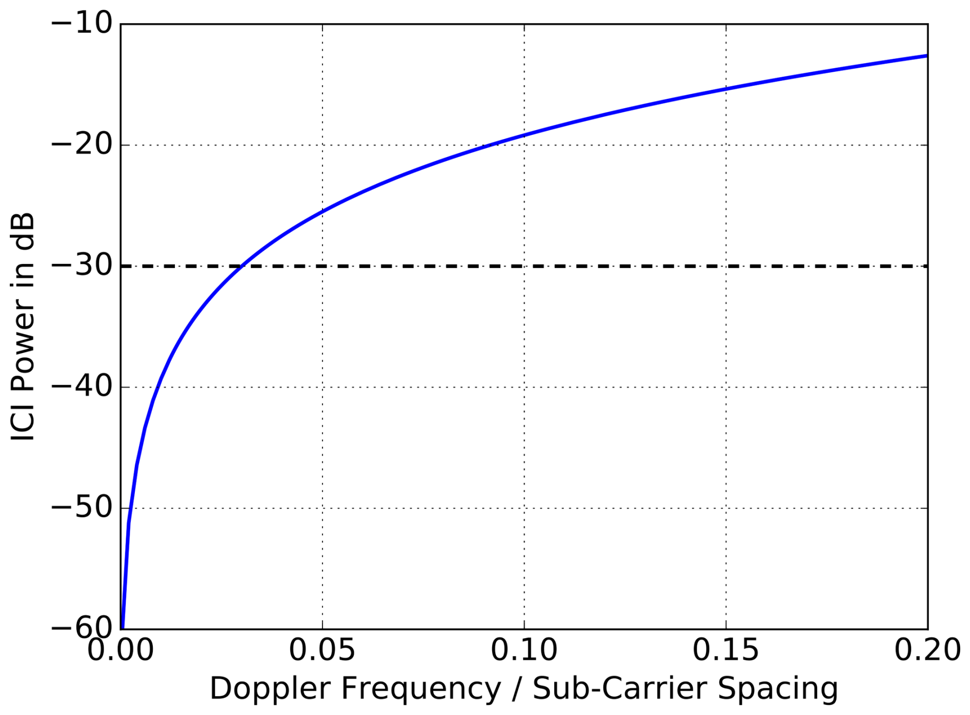
Figure 14 Inter-carrier-to-interference ratio of the OFDM signals with respect to the Doppler frequency normalized to the sub-carrier spacing ($\mathrm{\Delta }{f}_{\mathrm{Dop}}/\mathrm{\Delta }f$). The dotted line indicates the required ICI ratio.

Table 2 Overview of the waveform comparison.

5.4.3 OFDM Chirps

With respect to Doppler shifts, a significant drawback of OFDM signals is the interleaving behavior of the sub-carriers. Due to the small separation, given by Δf in Eq. (6), only a small Doppler bandwidth and thus a low azimuth resolution can be tolerated. In SAR applications, the individual sub-carriers are shifted due to the moving scene. This means that they are no longer orthogonal and cause interference between the signals. To analyze the amount of interference, the Inter-Carrier-to-Interference (ICI) ratio P_ICI has been defined (Kim et al., 2015):

$$\begin{array}{}\text{(28)}& P_{\mathrm{ICI}}=\underset{-\mathrm{\infty }}{\overset{\mathrm{\infty }}{\int }}\left(\mathrm{1}-{\text{sinc}}^{\mathrm{2}}\left(\mathit{\pi }\mathrm{\Delta }{f}_{\mathrm{Dop}}{\mathit{\tau }}_{\mathrm{p}}\right)\right)\cdot p_{\mathrm{d}}\left(\mathrm{\Delta }{f}_{\mathrm{Dop}}\right)\text{d}{f}_{\mathrm{Dop}}\end{array}$$

where p_d(Δf_Dop) is the Doppler probability density function (pdf). Described in words, it is the ratio of the power of an arbitrary reference sub-carrier to the total power of the interfering sub-carriers at that frequency. A plot of this ratio is shown in Fig. 14 with respect to the Doppler frequency normalized to the sub-carrier spacing ($\mathrm{\Delta }{f}_{\mathrm{Dop}}/\mathrm{\Delta }f$). For example, for a signal duration of τ_p=100 µs, using Eq. (6) we get Δf=10 kHz. Using the literature value of a maximum Doppler tolerance of $\mathrm{1}/\mathrm{10}\mathrm{\Delta }f$, the maximum acceptable Doppler bandwidth in our example must be less than 1 kHz. It turns out that this value is significantly lower than the required limit of 7.0 kHz and the sub-carrier will interfere strongly. Since these interferences affect the Noise Equivalent Sigma Zero (NESZ), cf. Krieger (2014), this value is definitely not acceptable. To ensure MIMO-SAR operation, an ICI of at least −30 dB is required, which leads to a maximum Doppler tolerance of only $\mathrm{1}/\mathrm{17}\mathrm{\Delta }f$ (also in agreement with Kim et al., 2015). For our example with Δf=10 kHz this means a maximum acceptable Doppler bandwidth of Δf_Dop=588 Hz, or an equivalent azimuth resolution of 12 m. Finally, OFDM has only limited applicability to MIMO-SAR and is only suitable to low or medium resolution SAR imaging.

5.5 Down-Link Issues

Nowadays, generating arbitrary waveforms with digital hardware is not a problem, but post-processing on-board the satellite is a demanding issue. Due to the limited data rate from the satellite to the ground station, it is necessary to pre-process the received multi-channel raw-data on-board. While the MSP and SSC waveforms can be processed in real-time on-board the satellite using the algorithm proposed in Rommel (2018), the OFDM chirp signals require a complex signal separation processing (Kim, 2011). The processing strategy proposed by Wang for the Chirp Diverse waveforms is a simple range compression with the corresponding transmit signal (Wang, 2015) as in typical SAR. It turns out that this is a significant advantage of this waveform type, although it has many other drawbacks.

6 Conclusions and summary

The increasing demand for High-Resolution Wide-Swath Synthetic Aperture Radar (HRWS-SAR) has spurred the development of sophisticated Digital Beamforming (DBF) and Multiple-Input Multiple-Output (MIMO) systems. In this context, the selection of optimal orthogonal waveforms remains a subject of intense debate with no general solution.

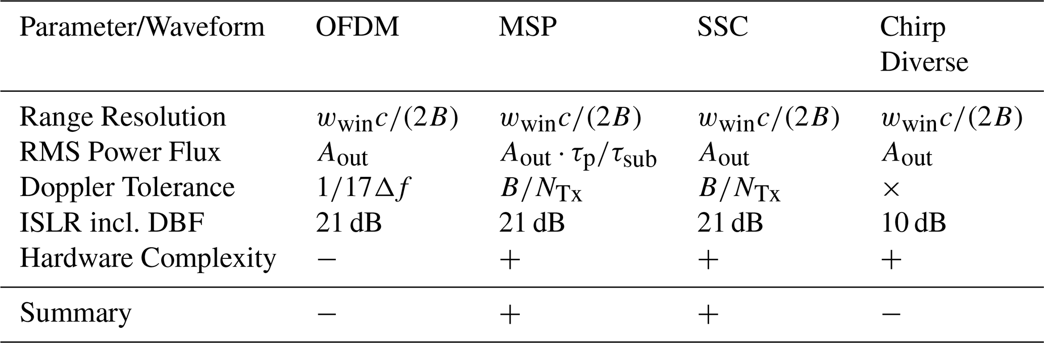
In this paper, we have comprehensively summarized and investigated various waveforms, including Up- and Down-Chirp modulation, OFDM chirp signals, Multiple Sub-Pulses, Segmentally-Shifted Chirp waveforms, and Chirp Diverse waveforms, as potential candidates for MIMO-SAR applications. After conducting a thorough analysis that included performance metrics such as range resolution, Integrated Sidelobe Ratio (ISLR), transmit energy, Doppler tolerance, and the ambiguity function, we determined that Multiple Sub-Pulses and Segmentally-Shifted Chirp waveforms are the best candidates for MIMO-SAR implementation due to their superior performance and reduced implementation complexity. The OFDM waveform could also be considered as an acceptable compromise for medium or low resolution systems. The MSP and SSC waveforms exhibit compatibility without introducing spurious interference, as summarized in Table 2. It must be noted that the row with the ISLR values assumes a tailored DBF to remove the step-wise rise (cf. Fig. 13), thus the optimal values of Table 1.

In the absence of a definitive decision rule or a universally superior waveform type, the comprehensive overview presented in this paper serves as a guideline, allowing engineers and researchers to make informed choices based on the specific sensor system and its primary requirements. Because technological advances may introduce new waveform types in the future, the criteria outlined here provide a robust framework for the analyzing and evaluating emerging waveform types.