Forcing mechanisms of the 6 h tide in the mesosphere/lower thermosphere

Solar tides such as the diurnal and semidiurnal tide, are forced in the lower and middle atmosphere through the diurnal cycle of solar radiation absorption. This is also the case with higher harmonics like the quarterdiurnal tide (QDT), but for these also non-linear interaction of tides such as the self-interaction of the semidiurnal tide, or the interaction of terdiurnal and diurnal tides, are discussed as possible forcing mechanism. To shed more light on the sources of the QDT, 12 years of meteor radar data at Collm (51.3^∘ N, 13^∘ E) have been analyzed with respect to the seasonal variability of the QDT at 82–97 km altitude, and bispectral analysis has been applied. The results indicate that non-linear interaction, in particular self-interaction of the semidiurnal tide probably plays an important role in winter, but to a lesser degree in summer. Numerical modelling of 6 h amplitudes qualitatively reproduces the gross seasonal structure of the observed 6 h wave at Collm. Model experiments with removed tidal forcing mechanisms lead to the conclusion that, although non-linear tidal interaction is one source of the QDT, the major forcing mechanism is direct solar forcing of the 6 h tidal components.

1 Introduction

The mesosphere and lower thermosphere (MLT) dynamics are strongly influenced by atmospheric waves, including the solar tides with periods of a solar day and its harmonics. Their wind amplitudes usually maximize around 100–120 km. At these heights, their amplitudes are comparable with the mean wind. Thus, the solar tides are an intrinsic part of the global circulation and more accurate knowledge of tides leads to a better understanding of the wind fields in the MLT in general. Shorter period tides often have smaller amplitudes, so that in the past especially the diurnal tide (DT), the semidiurnal tide (SDT), and also the terdiurnal tide (TDT) have been considered in investigations. The quarterdiurnal tide (QDT), however, although it also forms an integral part of the middle and upper atmosphere dynamics, has attained much less attention, mainly due to its small amplitude in the MLT. Near the surface the 6 h oscillation at times can be a major wave component as seen e.g. in barographic records (e.g., Warburton and Goodkind, 1977), but the 6 h amplitude in the MLT is generally substantially smaller than the one of the DT, SDT, and TDT. Consequently, only few attempts to determine the MLT QDT characteristics from radar or satellite observations have been made so far, and very few studies included the modelling of the QDT global structure and its sources.

Considerable QDT amplitudes have been reported by Walterscheid and Sivjee (1996, 2001) in the high-latitude winter, but they concluded that these were not migrating but zonally symmetric tides. From medium frequency radar winds over Adelaide, Australia and Davis, Antarctica, Kovalam and Vincent (2003) found signatures of 6 and 8 h tides, but belonging to a wavenumber 1 tide, so that they concluded that these oscillations are not thermally forced but possibly owing to non-linear interactions. Smith et al. (2004) investigated the QDT over Esrange, Sweden, and found that the QDT wind amplitudes on a monthly average may exceed 5 m s⁻¹ at 97 km altitude, and that they maximize in winter. Smith et al. (2004) also performed numerical simulations that revealed that much of the wintertime QDT is forced by the 6 h harmonic of solar heating, but without direct forcing the tide still appears and also maximizes in winter. Without direct solar forcing, the nonmigrating tidal modes became proportionally larger. Jacobi et al. (2017) used Collm (51.3^∘ N, 13.0^∘ E) meteor radar data. Their observed amplitudes and their seasonal cycle were similar to the ones presented by Smith et al. (2004). Comparison with radar observations at Obninsk, Russia, also indicated that most of the QDT signal at midlatitudes is probably due to its migrating components. Liu et al. (2006) noted a 6 h signature in medium frequency radar data over Wuhan, China, but mainly in their upper height gates above 90 km. They found from bispectral analyses that there are indications for non-linear interaction of tides as a possible forcing mechanism, but only in the upper height gates.

The 6 h harmonics of ozone heating rates have been calculated from Aura/MLS observations by Xu et al. (2012), who noted that the main 6 h forcing during solstice is in the winter hemisphere. Xu et al. (2014) analyzed nonmigrating tides from TIMED/SABER satellite observations. They confirmed earlier results that the QDT is largest in winter, and found indications that the nonmigrating QDT is likely to be forced by non-linear interaction between the DT and TDT, while the interaction between stationary planetary waves and the QDT is weak, likely because of the small amplitudes of the migrating QDT. In a further study, Liu et al. (2015), again using TIMED/SABER data, analyzed the migrating QDT between 50^∘ S and 50^∘ N in the middle atmosphere. From their analyses they considered both direct heating and tidal interaction as possible sources of the QDT. Azeem et al. (2016) analyzed observation from RAIDS/NIRS instruments, which confirmed solar heating as main source for the 6 h tide. But also other sources like non-linear interaction between tides could not be excluded.

Figure 1 Two examples of bicoherence spectral power as possible indicator for non-linear interaction. Analyzed data are half-hourly means at 91 km for (a) March 2005 (left) and (b) October 2014 (right). Only significant peaks are shown.

To summarize, to date there are rather few analyses of the QDT both locally and on a global scale, and in particular the forcing mechanisms of the QDT are still unclear and should be investigated further. Therefore, in the following we use the Collm data presented by Jacobi et al. (2017) and apply bispectral analysis to obtain indicators for possible forcing through non-linear interaction. In addition, we use a mechanistic numerical model and analyze the most likely forcing mechanism for the QDT through removing either solar heating or non-linear interaction for the model

2 Bispectral analysis of Collm meteor radar winds

The horizontal winds over Collm (51^∘ N, 13^∘ E) have been estimated from measurements obtained by a SKiYMET meteor radar, which is operated on 36.2 MHz since summer 2004. Details of the radar and the radial wind determination principle can be found in Jacobi (2012) and Stober et al. (2012). An update of the radar was performed in 2015, but without change of the transmit frequency (Stober et al., 2017). The individual meteor trail reflection heights vary between about 75 and 110 km, with a maximum meteor count rate around 90 km (e.g., Stober et al., 2008). The data are binned in 6 different not overlapping height gates, which are centred at 82, 85, 88, 91, 94, and 98 km. Meteors show a vertical distribution with increasing/decreasing count rates with height below/above 90 km, so that the nominal heights do not necessarily correspond to the mean heights. Therefore, below/above 90 km mean heights tend to be higher/lower than nominal heights and in particular the real mean height of the uppermost height gate is closer to 97 rather than 98 km. For the other height gates, the difference between real and nominal height is small (Jacobi, 2012).

Individual radial winds calculated from the meteors are collected to form half-hourly mean values using a least-squares fit of the horizontal wind components to the raw data under the assumption that vertical winds are small (Hocking et al., 2001). Tidal wind parameters at each height gate have been calculated by applying a least-squares regression analysis of one month of either zonal or meridional half-hourly horizontal winds on a model wind field including mean wind and tidal oscillations (Jacobi et al., 2017).

Bispectral analysis has proved to be a powerful tool to detect quadratic phase coupling between 3 frequencies. A bispectrum B(ω₁,ω₂) is nonzero for triplets of frequencies ${\mathit{\omega }}_{\mathrm{1}},{\mathit{\omega }}_{\mathrm{2}},{\mathit{\omega }}_{\mathrm{3}}$, when one of them is the sum or difference of the others, and there is phase coherence. Since non-linear interaction between tidal components result in exactly such a phase and frequency relationship, peaks in the bispectra can be used to detect possible non-linear interaction. Note however, that bispectra do not provide a real proof of non-linear interaction, because phase and frequency triplets could accidentally arise due to other reasons. The bispectrum may be written as:

$$\begin{array}{ll}{\displaystyle }B\left({\mathit{\omega }}_{\mathrm{1}},{\mathit{\omega }}_{\mathrm{2}}\right)=& {\displaystyle }\sum _{{\mathit{\tau }}_{\mathrm{1}}=-\mathrm{\infty }}^{\mathrm{\infty }}\sum _{{\mathit{\tau }}_{\mathrm{2}}=-\mathrm{\infty }}^{\mathrm{\infty }}{c}_{\mathrm{3}}\left({\mathit{\tau }}_{\mathrm{1}},{\mathit{\tau }}_{\mathrm{2}}\right)\\ \text{(1)}& {\displaystyle }& {\displaystyle }\cdot \exp \left\{-j\left({\mathit{\omega }}_{\mathrm{1}}{\mathit{\tau }}_{\mathrm{1}}+{\mathit{\omega }}_{\mathrm{2}}{\mathit{\tau }}_{\mathrm{2}}\right)\right\},\end{array}$$

with the third-order cumulant

$$\begin{array}{}\text{(2)}& {\displaystyle }{c}_{\mathrm{3}}\left({\mathit{\tau }}_{\mathrm{1}},{\mathit{\tau }}_{\mathrm{2}}\right)=E\left[v\left(k\right)v\left(k+{\mathit{\tau }}_{\mathrm{1}}\right)v\left(k+{\mathit{\tau }}_{\mathrm{2}}\right)\right],\end{array}$$

where v(k) are the individual detrended wind values and E is the expectancy value (Nikias and Raghuveer, 1987). For calculating the bispectral estimate of a finite record, the datasets are subdivided into K records with M samples. K and M should be as large as possible to reduce the large variance of the bispectral estimate and the phase coherence, which occurs by chance. For short data sets overlapping windows should be used to get enough segments (Lii and Helland, 1981). We used records of four days, i.e. M=192 half-hourly means, with a 50 % overlap, resulting in K=14 for one month (13 for February). A Hanning window was used. We apply the squared bicoherence spectrum b²(ω₁,ω₂) after Kim and Powers (1978) to estimate the fraction of power that is generated by quadratic phase coupling. It uses the power spectrum P(ω) for normalization and is suitable to examine frequency triplets, which show peaks in the power or amplitude spectrum:

$$\begin{array}{}\text{(3)}& {\displaystyle }{b}^{\mathrm{2}}\left({\mathit{\omega }}_{\mathrm{1}},{\mathit{\omega }}_{\mathrm{2}}\right)={\displaystyle \frac{{\left|B\left({\mathit{\omega }}_{\mathrm{1}},{\mathit{\omega }}_{\mathrm{2}}\right)\right|}^{\mathrm{2}}}{P\left({\mathit{\omega }}_{\mathrm{1}}\right)P\left({\mathit{\omega }}_{\mathrm{2}}\right)P\left({\mathit{\omega }}_{\mathrm{1}}+{\mathit{\omega }}_{\mathrm{2}}\right)}}.\end{array}$$

Two examples of zonal wind bicoherence spectra are shown in Fig. 1, one of them indicating a possible self-interaction of the SDT (Fig. 1a), the other one indicating coupling of the TDT and DT, and both resulting in a 6 h component.

In order to estimate, during which month of the year and at which altitude significant non-linear interaction is likely to occur, we estimated the 95 % significance level of bispectral peaks after Haubrich (1965) using $b^{\mathrm{2}}\ge \mathrm{6}/\mathrm{dof}$ as a conservative estimate (Elgar and Guza, 1985), with the degrees of freedom dof = 2 K. Actually, overlapping the records influences dof, which can be used to balance the effect of windowing the data records before the analysis (Emery and Thomson, 2001). Then, for each month of the year and for each height gate we calculated the number of years when we found significant spectral peaks for possible TDT/DT interaction and SDT self-interaction. Dividing this number by 12 resulted in a percentage of years, so that this shows how frequently there is an indication for significant non-linear interaction at this height and month. Figure 2 shows the percentage of years with significant peaks indicating self-interaction of the SDT (upper row) and interaction of the DT and TDT (lower row) in colour coding. In addition, the 12-year mean monthly mean tidal amplitudes are shown as contours. During winter, significant SDT self-interaction is frequently seen especially in the upper height gates (Fig. 2a, b). This generally coincides with maxima of the QDT, but also of the SDT which maximizes during winter (e.g. Jacobi, 2012). A secondary seasonal maximum of possible significant SDT self-interaction is found during autumn equinox, when the SDT also has a maximum (Jacobi, 2012). Significant bispectral peaks from interaction of the DT and TDT are less frequent (Fig. 2c, d). This kind of interaction has more effect during spring and autumn, when both the TDT and the DT have their maxima (Jacobi, 2012). The spring maximum of TDT/DT interaction is connected with a secondary maximum of QDT amplitudes, which is, however, only weakly visible during autumn also.

Figure 2 Colour coding: percentage of significant bicoherence peaks for the SDT self-interaction (panels a, b, upper row) and the TDT/DT interaction (panels c, d, lower row) for the zonal (panels a, c, left) and meridional (panels b, d, right) winds. Database are monthly data from 2005–2016 for each month of the year and for different heights. 12-year mean monthly mean amplitudes are added as contour lines.

To conclude, there is indication for significant non-linear interaction both of the SDT and of the TDT/DT, and these are more frequent during the months when the respective tidal components have large amplitudes. During these months maxima of the QDT are observed as well.

3 MUAM numerical model experiments

Since bispectral analysis neither provides a real proof for non-linear interaction nor gives quantitative measures how strong such a wave forcing would be, we performed numerical experiments using the Middle and Upper Atmosphere Model (MUAM, Pogoreltsev et al., 2007) to analyze the influence of different QDT forcing terms like direct solar heating and non-linear interaction at the latitude of the Collm radar observations. MUAM is a non-linear primitive equation mechanistic model of the atmospheric circulation with a resolution of 5^∘ × 5.625^∘ in the horizontal. In 56 vertical layers it extends up to a log-pressure height z of 160 km, which is given by $z=H\ln (p_{\mathrm{0}}/p)$ with p₀=1000 hPa and a scale height H=7 km. For time integration, a Matsuno (1966) scheme has been applied with a time step of 225 s. The model does not account for tropospheric effects such as orography or latent heat release. Therefore, the zonal mean temperature below 30 km is nudged with monthly mean ERA-Interim temperature fields in order to provide realistic dynamical features in the lower atmosphere.

Heating of the atmosphere due to absorption of solar radiation by water vapour, carbon dioxide, ozone, oxygen and nitrogen is introduced in the model via a radiation parameterization after Strobel (1981) (see also Fröhlich et al., 2003). The ozone and water vapour fields are prescribed as zonal means, so that mainly migrating tides are reproduced in the model. Infrared cooling of carbon dioxide is parameterized after Fomichev et al. (1998), while ozone infrared cooling in the 9.6 µm band is calculated after Fomichev and Shved (1985). Gravity waves in the middle atmosphere are parameterized according to a linear scheme as described by Fröhlich et al. (2003).

Zonal and meridional wind amplitudes of the modelled QDT at 52.5^∘ N (the nearest grid point to the Collm latitude) have been obtained from a frequency-wavenumber analysis of the migrating tides from one month of modelled data at each latitude and height level separately. They are shown in Fig. 3a, b. As in the observations, the meridional component is somewhat smaller than the zonal one. The zonal and meridional amplitudes maximize during February/March and November. Smaller maxima show up in May and July. The meridional component shows maxima also in February and March, as well as in October and November, but also during the summer months. The modelled amplitudes are generally smaller than the observed ones. This may be due to the fact that we only analyze migrating tides in the model. It has to be mentioned, however, that Jacobi et al. (2017) did not find evidence for a strong nonmigrating QDT so that their contribution to the total amplitude should not be as large as the difference between model and observations. The used model version does not include latent heat release in the troposphere, which also forces tidal components, and this may explain part of the reduced amplitudes. The observed seasonal cycle of the observed tide, however, is reproduced in general, except for another minimum near winter solstice, which is only weakly seen in the observations (Fig. 2, and Figs. 7 and 8 of Jacobi et al., 2017). The observed spring maxima are shifted a bit towards the summer.

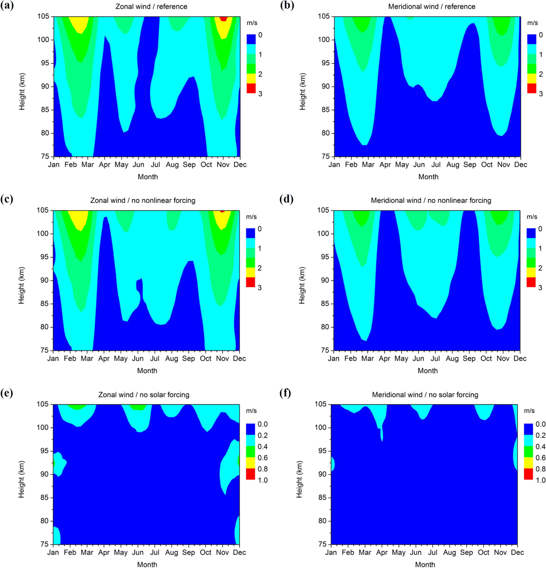
Figure 3 Modelled monthly mean QTD zonal (a, c, e) and meridional (b, d, f) amplitudes. The upper row shows results from reference runs. The second row shows results of runs with removed zonal wavenumber 4 components of non-linear interactions. The lowermost row shows results of runs with removed wavenumber 4 component of the solar forcing. Note the different colour coding of the lowermost panels.

To analyze the contribution of solar and non-linear forcing on the QDT amplitudes at higher midlatitudes, we removed the zonal wavenumber 4 component, which in the present configuration of the model is equivalent to the migrating QDT, from either (i) the non-linear terms of the prognostic equations or (ii) from the solar heating. The method of removing wavenumber components in the different forcing terms has been described in Lilienthal et al. (2018). Note that we only modelled migrating tidal components, so our results cannot be compared, e.g., with those of Xu et al. (2014). As Fig. 3c, d shows, the effect of removing non-linear terms is small and the QDT amplitudes are only weakly reduced. Partly, e.g. during midsummer, the amplitude increases slightly when non-linear forcing is removed. This is most likely an effect of destructive interference of the tidal components forced through absorption of solar radiation and by non-linear interaction. As Fig. 3e, f show, the remaining amplitudes after removing solar heating are small. This seasonal distribution is different from the observed one. An existence of non-linear forcing can be seen in December and January below 100 km, during the other months this is only the case at altitudes above 100 km.

4 Conclusions

Bispectral analysis of observed MLT winds at Collm indicate that non-linear interaction of tides may play a role in forcing the QDT. The major effect seen in the radar observations is due to self-interaction of the SDT, while interaction of the DT and TDT contribute to the QDT in spring and autumn. However, the fact that there are indications for non-linear interaction does not necessarily mean that the resulting QDT amplitudes are really strong. Indeed, MUAM model experiments show that, although there exists possible non-linear forcing of the QDT through tidal interaction, the resulting amplitudes are small, while the quarterdiurnal component of solar heating is the dominant forcing mechanism of the migrating QDT at the Collm latitude.

Of course the observations and model results cannot be compared directly. The main difference is that local radar measurements deliver the full amplitude, i.e. migrating and nonmigrating tides together, and separating is not possible from one observation alone. Furthermore, the MUAM model only provides reduced amplitudes, and does, for example, not show components due to latent heat release. In addition, the latitudinal resolution of the model is 5^∘, but the meridional structure of the QDT and its forcing is rather complex (e.g. Smith et al., 2004; Xu et al., 2012) so that a higher meridional model resolution may provide more accurate results.

The results presented here are all based on monthly mean analyses. Tides, however, are known to vary also at the day-to-day time scale, e.g. through their interaction with planetary waves. Therefore, it is possible that at time scales shorter than one month, the SDT, TDT, or DT are increased and non-linear interactions leading to a QDT signature would be stronger in relation to solar forcing. While analyzing this is beyond the scope of this paper and would require a modified modelling approach including e.g. the analysis of planetary waves, a more comprehensive analysis of the QDT forcing at short time scales is certainly worthwhile and should be performed in further studies. Finally, MUAM is a global model and thus global results of QDT forcing can be obtained, but satellite observations will be necessary for validation of the results. Therefore, in future analyses, we plan to extend the model analysis and use QDT amplitude distributions from GPS radio occultations (e.g. Arras and Wickert, 2017) for validiation.