 | 04 Sep 2018
Ionospheric response to solar EUV variations: Preliminary results
Rajesh Vaishnav
Christoph Jacobi
Jens Berdermann
Erik Schmölter
Mihail Codrescu
We investigate the ionospheric response to solar Extreme Ultraviolet (EUV) variations using different proxies, based on solar EUV spectra observed from the Solar Extreme Ultraviolet Experiment (SEE) onboard the Thermosphere Ionosphere Mesosphere Energetics and Dynamics (TIMED) satellite, the F10.7 index (solar irradiance at 10.7 cm), and the Bremen composite Mg-II index during January 2003 to December 2016. The daily mean solar proxies are compared with global mean Total Electron Content (GTEC) values calculated from global IGS TEC maps. The preliminary analysis shows a significant correlation between GTEC and both the integrated flux from SEE and the Mg II index, while F10.7 correlates less strongly with GTEC. The correlations of EUV proxies and GTEC at different time periods are presented. An ionospheric delay in GTEC is observed at the 27 days solar rotation period with the time scale of about ∼1–2 days. An experiment with the physics based global 3-D Coupled Thermosphere/Ionosphere Plasmasphere electrodynamics (CTIPe) numerical model was performed to reproduce the ionospheric delay. Model simulations were performed for different values of the F10.7 index while keeping all the other model inputs constant. Preliminary results qualitatively reproduce the observed ∼1–2 days delay in GTEC, which is might be due to vertical transport processes.
- Article
(3263 KB) - Full-text XML
- BibTeX
- EndNote


The ionospheric E and F regions are important layers of the Earth's atmosphere (above ∼60 km), which are created due to ionization of various species like nitrogen, atomic oxygen, and molecular oxygen. The ionosphere is built through absorbing solar extreme ultraviolet (EUV) radiation and soft X-rays mainly at wavelengths below 105 nm. The EUV radiation is not emitted at constant rates and varies at different timescales, including short-term variability (minutes (flares), daily, 27 days Carrington rotation, and seasonal) and long term variability (11 years solar cycle). The long term variability is expected to be greater than the short term variability (Woods and Rottman, 2002). For instance, the He II EUV emission line can change by a factor of 2 during the 11 years solar cycle and ∼50 % during the 27 days rotation period, and the variation in EUV can be 30 % at ∼100 nm and 100 % at ∼10 nm during the solar rotation period (e.g. Lean et al., 2001, 2011). During solar flares, the X-rays and the solar EUV regions may be enhanced by more than a factor of 50 and less than a factor of 2, respectively (Woods and Eparvier, 2006). Short-term solar variability is part of space weather, so that ionospheric parameters like the Total Electron Content (TEC) and the ionospheric height (McNamara and Smith, 1982) are influenced by space weather. TEC is the vertically integrated electron density of the ionosphere which is usually given in TEC units (1 TECU = 1016electrons m−2). The ionospheric variability due to changes in solar activity has been studied extensively by various researchers (e.g., Jakowski et al., 1991; Rishbeth, 1993; Su et al., 1999; Forbes et al., 2000; Liu et al., 2006; Afraimovich et al., 2008; Lee et al., 2012; Jacobi et al., 2016, and references therein). Such studies are of great importance for improving our understanding of the solar influence on radio communication and navigation systems like Global Navigation Satellite Systems (GNSS). Radio waves are refracted by the ionosphere, which in turn is affected by the solar activity.
Due to unavailability of direct EUV measurements before the space age, the variation in TEC is frequently compared against solar proxies, with the most common one being the F10.7 index, which is the irradiance at a wavelength of 10.7 cm, usually given in solar flux units (sfu, 10−22 W m−2 Hz−1) (Tapping, 1987; Rishbeth, 1993; Maruyama, 2010). Other indices are the Bremen composite MG-II index (the core to wing ratio of the MG-II line) (Maruyama, 2010), or EUV-TEC which have been introduced by Unglaub et al. (2011) to name only a few. The long-term and short-term relation between EUV and different solar proxies (F10.7 index, Mg-II index, Sunspot number) has been reported in previous studies (Dudok de Wit et al., 2009; Chen et al., 2012; Wintoft, 2011). In comparison to the short term variability, the long-term variations of EUV radiation are better represented by the solar proxies (Chen et al., 2012). All the proxies not always perfectly describe the solar activity (Dudok de Wit et al., 2009), and their capability in reproducing EUV depends on wavelength and time scale. Chen et al. (2011) suggested that the F10.7 index is not able to produce the solar activity level during the minima of solar cycle 23, and Chen et al. (2012) showed that the MG-II index is a better representative of SOHO EUV in the wavelength range 26–34 nm than the F10.7 index. On the other hand, good correlation has been observed between ionospheric parameters and F10.7 index during Autumn–Winter of the years 2003 to 2005 (Oinats et al., 2008).
In recent years, direct solar EUV flux measurements are available from various satellites such as the Solar EUV Experiment (SEE) onboard the Thermosphere Ionosphere Mesosphere Energetics and Dynamics (TIMED) satellite (Woods et al., 2000, 2005), and the Extreme Ultraviolet Variability Experiment (EVE) onboard the Solar Dynamics Observatory (SDO) (Woods et al., 2012; Pesnell et al., 2012). However, due to degradation of EUV measuring instruments solar proxies may be more suitable (BenMoussa et al., 2013), or repeated calibration is necessary. The availability of the direct EUV measurements provide an opportunity for comparing EUV with different solar proxies (e.g., Jacobi et al., 2016).
Various researchers had observed a delayed response of ∼1–2 days in TEC or global mean TEC (GTEC) with respect to solar activity changes (e.g. Jakowski et al., 1991; Oinats et al., 2008; Afraimovich et al., 2008; Min et al., 2009; Lee et al., 2012; Jacobi et al., 2016). Hocke (2008) showed the 11 years, 1 year, and 27 days oscillations of GTEC and the Mg-II index with a high correlation coefficient. Lee et al. (2012) studied the correlation and time lag at the 27 days solar rotation period using GPS TEC and in situ electron density measurements from the CHAMP and GRACE satellites. They found a 1-day difference of the time delay in the northern and southern hemisphere. Jakowski et al. (1991) used a 1-D numerical model to explain the delay of ∼1–2 days. The study concluded that the delay might be due to slow diffusion of atomic oxygen at 180 km, which was produced due to dissociation of molecular oxygen in the lower altitude.
In recent years numerical, empirical, and physics-based thermosphere/ionosphere models have been developed to characterize ionospheric dynamics. Among them are the Coupled Thermosphere Ionosphere Plasmasphere Electrodynamics (CTIPe, Fuller-Rowell and Rees, 1983; Millward et al., 2001; Codrescu et al., 2012), the International Reference Ionosphere (IRI, Rawer et al., 1978; Bilitza et al., 2011) and Thermosphere-Ionosphere-Electrodynamics General Circulation Model (TIE-GCM, Roble et al., 1988). These models play an important role in upper atmospheric studies (e.g., Negrea et al., 2012; Fedrizzi et al., 2012). To simulate solar variability, models are frequently driven by proxies like F10.7 index or the Mg-II index. The F10.7 index is the most widely used index in upper atmosphere research to represent the solar variability due to the availability of continuous measurements since 1947 (Woods et al., 2005). The solar EUV variability can be better represented by the improved F10.7 index using 81 days running mean (e.g., Viereck et al., 2001; Liu et al., 2006). The CTIPe model uses a modified F10.7 index, which is the average of the previous day value of the F10.7 index and the average of the previous 41 days (Codrescu et al., 2012). Fitzmaurice et al. (2017) used the CTIPe model to understand the influence of solar activity on the ionosphere/thermosphere during the geomagnetic storm. They reported that solar activity has the greatest effect on model simulated TEC.
The main aim of the present study is to find out the correlation and time delay between GTEC and solar proxies based on data from January 2003 to December 2016. To derive the periodicities in GTEC and solar proxies, the wavelet coherence and cross-wavelet method have been utilized. Preliminary results of a CTIPe model experiment to estimate the delay at the solar rotation time scale will also be presented.
2.1 Data sources
In this work, we use daily global TEC maps from the International GNSS Service (IGS, Hernandez-Pajares et al., 2009) provided by NASA's CDDIS (Noll, 2010) data archive service (CDDIS, 2017). Gridded global TEC data is available at a time resolution of 2 h and on a spatial grid of in latitude-longitude. For the analysis of the correlation between solar proxies and GTEC, we have selected three commonly used solar proxies, namely daily values of the F10.7 index, the Bremen composite Mg-II index, and the integrated EUV flux from the TIMED/SEE satellite. The F10.7 index and TIMED/SEE measurements are taken from the LISIRD (DeWolfe et al., 2010) database. The NASA TIMED satellite was launched in 2001 and carried four instruments (GUVI, SABER, SEE and TIDI). Solar irradiance measurements from the TIMED/SEE instrument are available since 22 January 2002 (Woods et al., 2005). The SEE instrument is designed to measure the soft X-rays and EUV radiation from 0.1 to 194 nm with the resolution and accuracy of 0.1 nm and ∼10–20 %, respectively. SEE includes two instruments, the EUV grating spectrograph and the XUV photometer system (Woods et al., 2000). We have used the daily integrated value of solar irradiance from 5.5 to 105.5 nm wavelength.
2.2 CTIPe model description

Figure 1Temporal variations of normalized datasets of GTEC (blue), SEE-EUV flux (black), F10.7 index (red), and Mg-II index (magenta) during year 2003 to 2016. The curves are vertically offset each by 2.
The CTIPe model is a global, 3-D, time-dependent, physics-based numerical model. It consists of four components, namely (a) a neutral thermosphere model (Fuller-Rowell and Rees, 1980), (b) a mid- and high-latitude ionosphere convection model (Quegan et al., 1982), (c) a plasmasphere and low latitude ionosphere model (Millward et al., 1996), and (d) an electrodynamics model (Richmond et al., 1992), which run simultaneously and are fully coupled. The thermosphere model is solving the equation of momentum, continuity, and energy to calculate global temperature, density, wind components, and atmospheric neutral composition. The parameters calculated from the thermosphere code are used to calculate production, loss, and transport of plasma. The transport terms consider ExB drift and interactions of ionised and neutral particles under the influence of the magnetospheric electric field (Codrescu et al., 2012). In the high latitude model, the atomic ions of O+ and H+ are calculated by solving the momentum, energy, and continuity equations, and the model includes vertical diffusion, horizontal transport, ion-ion, and ion neutral processes in the height range of 100 to 10 000 km. The contribution from N2+, O2+, NO+ and N+ are additionally added below 400 km. The mid and low latitude ionosphere model is also calculating H+, O+ ions, and electrons as does the high latitude model. The numerical solution of the composition equation with the energy and momentum equations describe the transport, turbulence, and diffusion of atomic oxygen, molecular oxygen and nitrogen (Fuller-Rowell and Rees, 1983). The latitude/longitude resolution is 2∘/18∘. In the vertical direction, the atmosphere is divided into 15 levels in logarithmic pressure starting from a lower boundary at 1 Pa to ∼500 km altitude at an interval of one scale height. The corresponding geometric heights are variable depending on temperature and therefore on the solar and magnetic activity. External inputs are required to drive the model like solar UV and EUV, Weimer electric field, TIROS/NOAA auroral precipitation, and tidal forcing. The F10.7 index is used in an artificial manner as input solar proxy to calculate ionization, heating, and oxygen dissociation processes in the ionosphere. For the simulation, the Hinteregger et al. (1981) reference solar spectrum driven by variations of input F10.7 is used in the model. More description of CTIPe is available in Codrescu et al. (2008, 2012).
3.1 Correlation between TEC and solar EUV proxies
To study the long-term variations in GTEC and EUV proxies, datasets from 2003 to 2016 have been used. Figure 1 shows the normalized time series of GTEC, SEE EUV flux, the F10.7 index, and the MG-II index. All data has been normalized by subtracting the mean and dividing by the respective standard deviation. The data represent the decreasing and increasing parts of solar cycle 23 and 24, respectively. As the solar radiation plays a major role in the electron production, the correlation of GTEC with solar EUV or EUV proxies must be significant and is also correlated at the 27 days solar rotation period. Figure 2 shows the cross correlation between GTEC and (a) TIMED/SEE integrated EUV flux (left panel), and (b) F10.7 index (right panel) from 1 January 2003 to 31 December 2016. Since we do not consider the seasonal cycle here, a low-pass filter with a cut off period of three months was applied to the data before.
Figure 2 shows a strong correlation between normalized GTEC and integrated EUV flux (black) with a maximum correlation coefficient of 0.90 and shows a weaker correlation with the F10.7 index (red) with a maximum correlation coefficient of 0.84. Also, we have analyzed the correlation between GTEC and Mg-II index which shows a good correlation with a correlation coefficient of 0.89 (figure not shown). Jacobi et al. (2016) analyzed GTEC and SDO/EVE integrated EUV flux data from 2011 to 2014 and they also found a good correlation of about 0.89. Unglaub et al. (2011, 2012) have shown that the GTEC is more strongly correlated with the EUV-TEC proxy than with the F10.7 index. Figure 2 shows a delay of ∼1–2 days in GTEC with respect to both SEE flux and F10.7 index, which confirms earlier analyses e.g. by Jacobi et al. (2016).

Figure 2Cross-correlation of GTEC with SEE-EUV flux (black) and F10.7 index (red). Positive values denote GTEC lagging SEE-EUV or F10.7, respectively.
3.2 Wavelet analysis
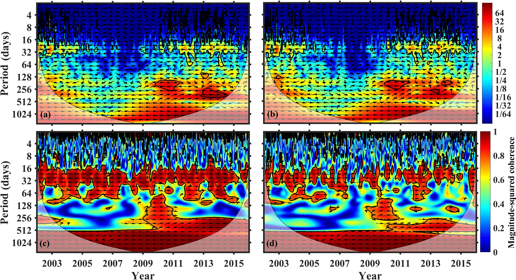
Figure 3(a, b): cross-wavelet transform of the GTEC with (a) SEE-EUV flux and (b) F10.7 index. (c, d): wavelet coherence of the GTEC with (c) SEE-EUV flux and (d) F10.7 index. The cone of influence is shown by a black line. Significant values are surrounded by a black line. The arrows show the phase relationship: in-phase pointing right, anti-phase pointing left, while downward direction means that GTEC is leading.
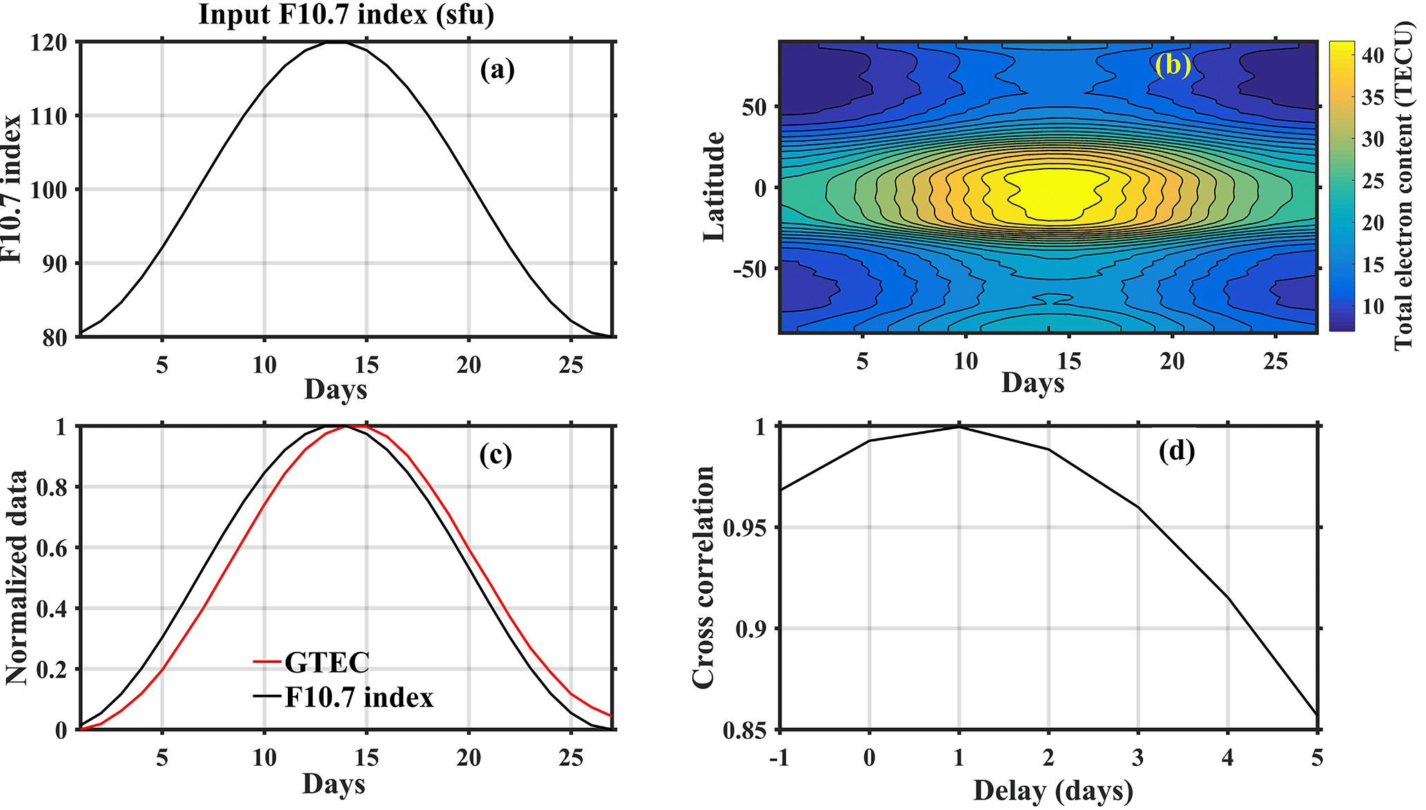
Figure 4(a) input F10.7 index values for CTIPe model simulation, (b) simulated zonal mean TEC, (c) normalized data of F10.7 index and modelled GTEC, and (d) cross-correlation between F10.7 index and modelled GTEC.
In order to investigate the oscillations in the time series of GTEC and all EUV proxies in more detail, the continuous wavelet transform (CWT) method has been applied. The cross wavelet transform is constructed using 2 CWTs, which shows common high energies of the two time series and relative phase (Grinsted et al., 2004). We have used a Morlet mother wavelet. Furthermore, the wavelet coherence method is used to calculate significant coherence using Monte Carlo methods (Grinsted et al., 2004). Wavelet coherence can be calculated using 2 CWTs which shows the local correlation between the time series. All data has been normalized by subtracting the mean and dividing by the respective standard deviation.
The cross wavelet spectra between GTEC and both SEE–EUV flux and F10.7 index are shown in Fig. 3a and b, respectively.
GTEC shows common high power with SEE-EUV flux and F10.7 at scales of 16–32 days during 2003 to 2005 and during 2009 to 2016. During those times when the coherence is significant, GTEC is in phase with SEE-EUV and F10.7. Much less power at the 27 days periodicity is observed from 2007 to 2009, which is the extended part of solar cycle 23.
The magnitude squared coherence of GTEC with SEE-EUV flux and the F10.7 index is shown in Fig. 3c and d, respectively. The coherence spectrum shows the time and period range where the two time series co-vary. As shown in both figures, a high correlation is observed at the 27 days periodicity. The magnitude squared coherence between GTEC and SEE flux is very high at 27 days periodicity, while GTEC and F10.7 behave less coherent. In comparison to the cross wavelet in Fig. 3a, b, wavelet coherence shows larger significant regions in Fig. 3c, d.
3.3 Variation in TEC using varying F10.7 values in CTIPe model
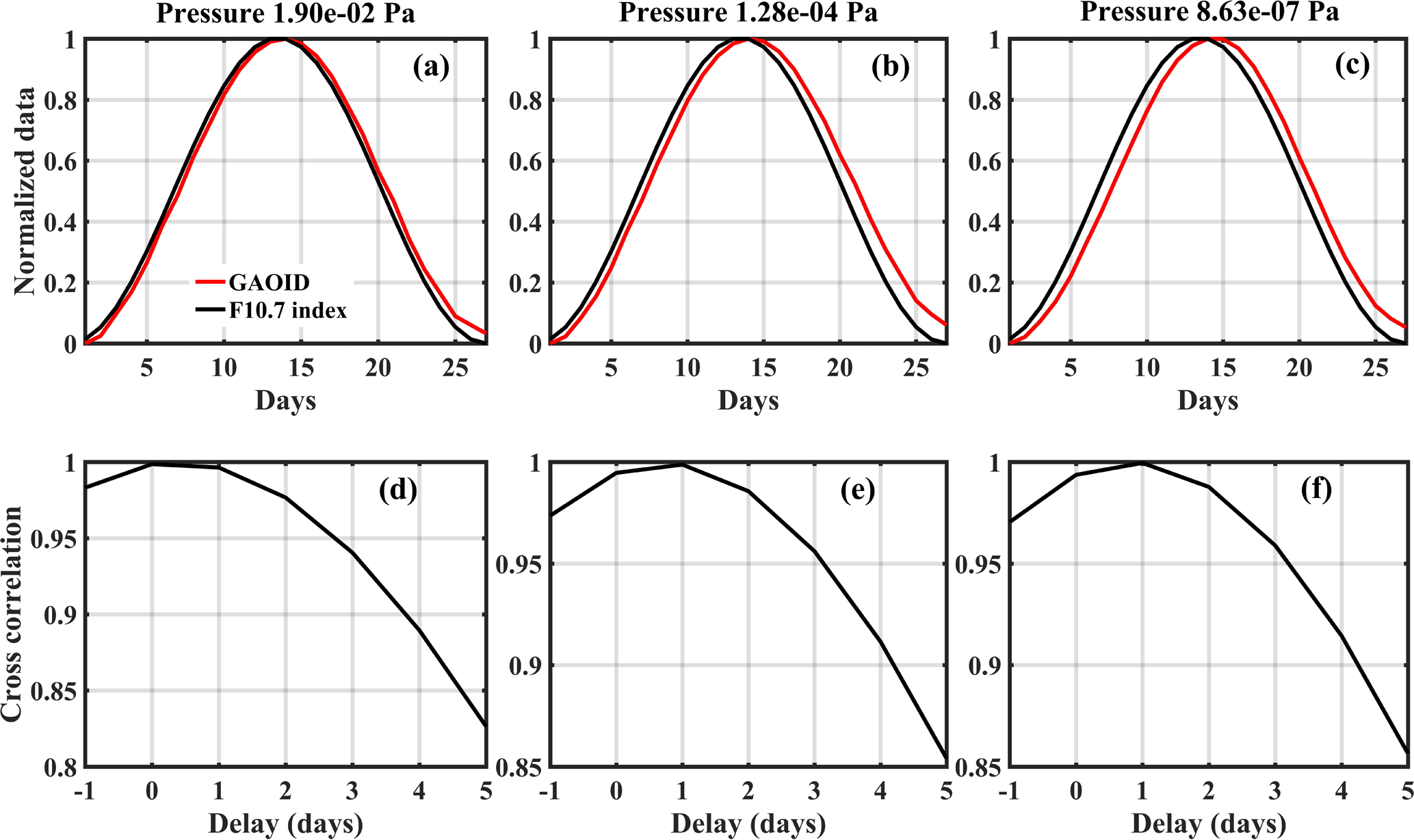
Figure 5(a, b, c): Normalized modelled GAOID and input F10.7 data at three different pressure levels. (d, e, f): Corresponding cross-correlations between F10.7 and modelled GAOID.
The CTIPe model has been used to simulate the ionospheric variability and to estimate the ionospheric delay due to solar variability. The model was run for 15 March 2013 conditions (Kp index = 3) and simulates TEC by varying the F10.7 index values in an artificial manner as input, keeping all the other input parameters constant. The input lower boundary in the CTIPe model is specified by the output of the Whole Atmospheric Model (WAM) (Akmaev, 2011). For the experiment, the model was first run for 30 days with constant input to reach a diurnally reproducible global temperature pattern, and then F10.7 was modified. Figure 4a shows the chosen F10.7 index values as input for the model, which vary from 80 to 120 sfu during one complete solar rotation period.
Figure 4b shows the zonal mean TEC simulated by the CTIPe model. The global TEC distribution qualitatively reproduces real ionospheric conditions, e.g. enhanced electron density near the equator due to the fountain effect (Appleton, 1946; Hanson and Moffett, 1966; Sterling et al., 1969). TEC varies according to the F10.7 index, but with a delay which can be seen by comparing the TEC maximum with the one of F10.7 in Fig. 4a. Figure 4c shows global mean values for the F10.7 index and the CTIPe TEC, both normalized by subtracting the mean and dividing by the respective standard deviation. A delay of about 1–2 days is observed. Figure 4d shows the cross-correlation and thus the delay between the input F10.7 index and TEC simulated by the CTIPe model. The delay introduced here may be due to vertical transport processes or slow diffusion of atomic oxygen, which has been suggested by Jakowski et al. (1991) as a possible process for the ionospheric delay. In order to understand the possible delay mechanism in the GTEC, the normalized modelled global mean atomic oxygen ion density (GAOID) is shown in Fig. 5 (upper row) for different altitudes. The corresponding cross correlations between the F10.7 index and GAOID are shown in the lower panel. It is interesting to note that at pressure Pascal in Fig. 5d there is only a small delay in GAOID with respect to F10.7, but Fig. 5b, e and c, f show a larger delay of ∼1 day at greater altitudes. This preliminary analysis indicates that vertical transport processes might play a role in the delay.
To contribute to the understanding of the long-term ionospheric behaviour with respect to solar EUV variations we have analyzed data from 1 January 2003 to 31 December 2016. In this study, the strong correlation between GTEC and solar proxies has been observed at the 27 days solar rotation period. There is a particularly strong correlation between GTEC and integrated SEE-EUV flux and the Mg II index, while F10.7 correlates less strongly with TEC. We have also observed an ionospheric delay at the 27 days solar rotation period with the time scale of 1–2 days between GTEC and all the solar proxies considered, thereby confirming earlier results in the literature.
To gain more insight into the possible reasons for the delay, we have run the CTIPe model for 27 days and varied the input F10.7 index artificially while keeping all the other conditions constant. Preliminary results show that the model qualitatively reproduces the observed ionospheric delay of ∼1–2 days in GTEC with respect to the F10.7 index. An attempt has been made to understand the delay process using GAOID simulated by the CTIPe. The cross correlation analysis between the GAOID and the F10.7 indicates small delay at the lower pressure level and longer delay in higher pressure levels, which suggests that transport processes might play a role in the delay.
To conclude, in this first approach we have found that the CTIPe model is able to reproduce the observed ionospheric delay. The results, however, are only preliminary. In further studies with more realistic EUV changes, we will also analyse photodissociation and ionization processes of atomic oxygen, molecular oxygen, and molecular nitrogen in more detail to check the validity of the results by Jakowski et al. (1991). Furthermore, we will investigate the delay in the different ionospheric parameters on different timescales by varying various model components (dissociation, ionization) thereby investigating the physical processes responsible for the delay.
IGS TEC data has been provided via NASA through ftp://cddis.gsfc.nasa.gov/gnss/products/ionex/ (CDDIS, 2017). Daily F10.7 index and TIMED/SEE version 3A spectra have been provided by LASP at http://lasp.colorado.edu/lisird/noaa_radio_flux and http://lasp.colorado.edu/lisird/data/timed_see_ssi_l3a (LASP, 2017), respectively. Mg-II index has been provided by IUP at http://www.iup.uni-bremen.de/UVSAT/Datasets/mgii (IUP, 2017).
CJ, RV, JB, ES, and MC designed the study. RV performed the CTIPe model run with help from MC and CJ. RV analysed the data. CJ together with RV drafted the first version of the text. All authors discussed the results and provided critical feedback and contributed to the final version of the manuscript.
The authors declare that they have no conflict of interest.
This article is part of the special issue “Kleinheubacher Berichte 2017”. It is a result of the Kleinheubacher Tagung 2017, Miltenberg, Germany, 25–27 September 2017
The study has been supported by Deutsche Forschungsgemeinschaft (DFG) through
grants no. BE 5789/2-1 and JA 836/33-1.
Edited by: Ralph Latteck
Reviewed by: Matthias Förster and
one anonymous referee
Afraimovich, E. L., Astafyeva, E. I., Oinats, A. V., Yasukevich, Yu. V., and Zhivetiev, I. V.: Global electron content: a new conception to track solar activity, Ann. Geophys., 26, 335–344, https://doi.org/10.5194/angeo-26-335-2008, 2008.
Akmaev, R. A.: Whole atmosphere modeling: Connecting terrestrial and space weather, Rev. Geophys., 49, RG4004, https://doi.org/10.1029/2011RG000364, 2011.
Appleton, E. V.: Two anomalies in the ionosphere, Nature, 157, 691, https://doi.org/10.1038/157691a0, 1946.
BenMoussa, A., Gissot, S., Schühle, U., Del Zanna, G., Auchère, F., Mekaoui, S., Jones, A. R., Walton, D., Eyles, C. J., Thuillier, G., Seaton, D., Dammasch, I. E., Cessateur, G., Meftah, M., Andretta, V., Berghmans, D., Bewsher, D., Bolsée, D., Bradley, L., Brown, D. S., Chamberlin, P. C., Dewitte, S., Didkovsky, L. V., Dominique, M., Eparvier, F. G., Foujols, T., Gillotay, D., Giordanengo, B., Halain, J. P., Hock, R. A., Irbah, A., Jeppesen, C., Judge, D. L., Kretzschmar, M., McMullin, D. R., Nicula, B., Schmutz, W., Ucker, G., Wieman, S., Woodraska, D., and Woods, T. N.: On-orbit degradation of solar instruments, Sol. Phys., 288, 389–434, https://doi.org/10.1007/s11207-013-0290-z, 2013.
Bilitza, D., McKinnell, L. A., Reinisch, B., and Fuller-Rowell, T.: The International Reference Ionosphere (IRI) today and in the future, J. Geodesy., 85, 909–920, https://doi.org/10.1007/s00190-010-0427-x, 2011.
CDDIS: GNSS Atmospheric Products, available at: http://cddis.nasa.gov/Data_and_Derived_Products/GNSS/atmospheric_products.html (last access: 29 June), 2017.
Chen, Y., Liu, L., and Wan, W.: Does the F10.7 index correctly describe solar EUV flux during the deep solar minimum of 2007–2009?, J. Geophys. Res., 116, A04304, https://doi.org/10.1029/2010JA016301, 2011.
Chen, Y., Liu, L., and Wan, W.: The discrepancy in solar EUV-proxy correlations on solar cycle and solar rotation timescales and its manifestation in the ionosphere, J. Geophys. Res., 117, A03313, https://doi.org/10.1029/2011JA017224, 2012.
Codrescu, M. V., Fuller-Rowell, T. J., Munteanu, V., Minter, C. F., and Millward, G. H.: Validation of the coupled thermosphere ionosphere plasmasphere electrodynamics model: CTIPe-Mass Spectrometer Incoherent Scatter temperature comparison, Adv. Space Res., 6, S09005, https://doi.org/10.1029/2007SW000364, 2008.
Codrescu, M. V., Negrea, C., Fedrizzi, M., Fuller-Rowell, T. J., Dobin, A., Jakowsky, N., Khalsa, H., Matsuo, T., and Maruyama, N.: A real-time run of the Coupled Thermosphere Ionosphere Plasmasphere Electrodynamics (CTIPe) model, Adv. Space Res., 10, S02001, https://doi.org/10.1029/2011SW000736, 2012.
DeWolfe, A. W., Wilson, A., Lindholm, D. M., Pankratz, C. K., Snow, M. A., and Woods, T. N.: Solar Irradiance Data Products at the LASP Interactive Solar Irradiance Datacenter (LISIRD), in: AGU Fall Meeting 2010, Abstract GC21B-0881, San Francisco, California, USA, 2010.
Dudok de Wit, T., Kretzschmar, M., Lilensten, J., and Woods, T.: Finding the best proxies for the solar UV irradiance, Geophys. Res. Lett., 36, L10107, https://doi.org/10.1029/2009GL037825, 2009.
Fedrizzi, M., Fuller-Rowell, T. J., and Codrescu, M. V.: Global Joule heating index derived from thermospheric density physics- based modeling and observations, Adv. Space Res., 10, S03001, https://doi.org/10.1029/2011SW000724, 2012.
Fitzmaurice, A., Kunznetsova, M., Shim, J. S., and Uritskey, V.: Impact of Solar Activity on the Ionosphere/Thermosphere during Geomagnetic Quiet Time for CTIPe and TIE-GCM, Arxiv, Physics eprint, arXiv:1701.06525, 2017.
Forbes, J. M., Palo, S. E., and Zhang, X.: Variability of the ionosphere, J. Atmos. Sol.-Terr. Phy., 62, 685–693, https://doi.org/10.1016/S1364-6826(00)00029-8, 2000.
Fuller-Rowell, T. J. and Rees, D.: A three-dimensional time-dependent global model of the thermosphere, J. Atmos. Sci., 37, 2545–2567, https://doi.org/10.1175/1520-0469(1980)037<2545:ATDTDG>2.0.CO;2, 1980.
Fuller-Rowell, T. J. and Rees, D.: Derivation of a conservation equation for mean molecular weight for a two-constituent gas within a three-dimensional, time-dependent model of the thermosphere, Planet. Space Sci., 31, 1209–1222, https://doi.org/10.1016/0032-0633(83)90112-5, 1983.
Grinsted, A., Moore, J. C., and Jevrejeva, S.: Application of the cross wavelet transform and wavelet coherence to geophysical time series, Nonlinear Proc. Geoph., 11, 561–566, https://doi.org/10.5194/npg-11-561-2004, 2004.
Hanson W. B. and Moffett, R. J.: Ionization transport effects in the equatorial F-region, J. Geophys. Res., 71, 5559–5572, https://doi.org/10.1029/JZ071i023p05559, 1966.
Hernandez-Pajares, M., Juan, J. M., Sanz, J., Orus, R., Garcia-Rigo, A., Feltens, J., Komjathy, A., Schaer, S. C., and Krankowski, A.: The IGS VTEC maps: a reliable source of ionospheric information since 1998, J. Geodyn., 83, 263–275, https://doi.org/10.1007/s00190-008-0266-1, 2009.
Hinteregger, H. E., Fukui, K., and Gilson, B. R.: Observational, reference and model data on solar EUV, from measurements on AE-E, Geophys. Res. Lett., 8, 1147–1150, https://doi.org/10.1029/GL008i011p01147, 1981.
Hocke, K.: Oscillations of global mean TEC, J. Geophys. Res., 113, 1–13, A04302, https://doi.org/10.1029/2007JA012798, 2008.
IUP: Mg-II index, available at: http://www.iup.uni-bremen.de/UVSAT/Datasets/mgii, last access: 30 June 2017.
Jacobi, C., Jakowski, N., Schmidtke, G., and Woods, T. N.: Delayed response of the global total electron content to solar EUV variations, Adv. Radio Sci., 14, 175–180, https://doi.org/10.5194/ars-14-175-2016, 2016.
Jakowski, N., Fichtelmann, B., and Jungstand, A.: Solar activity control of Ionospheric and thermospheric processes, J. Atmos. Terr. Phys., 53, 1125–1130, https://doi.org/10.1016/0021-9169(91)90061-B, 1991.
LASP (2017): LASP Interactive Solar Irradiance Data Center, available at: http://lasp.colorado.edu/lisird, last access: 30 June 2017.
Lean, J. L., White, O. R., Livingston, W. C., and Picone, J. M.: Variability of a composite chromospheric irradiance index during the 11-year activity cycle and over longer time periods, J. Geophys. Res., 106, 10645–10658, https://doi.org/10.1029/2000JA000340, 2001.
Lean, J. L., Woods, T. N., Eparvier, F. G., Meier, R. R., Strickland, D. J., Correira, J. T., and Evans, J. S.: Solar extreme ultraviolet irradiance: Present, past, and future, J. Geophys. Res., 116, A01102, https://doi.org/10.1029/2010JA015901, 2011.
Lee, C. K., Han, S. C., Bilitza, D., and Seo, K. W.: Global characteristics of the correlation and time lag between solar and ionospheric parameters in the 27-day period, J. Atmos. Sol-Terr. Phy., 77, 219–224, https://doi.org/10.1016/j.jastp.2012.01.010, 2012.
Liu, L., Wan, W., Ning, B., Pirog, O. M., and Kurkin V. I.: Solar activity variations of the ionospheric peak electron density, J. Geophys. Res., 111, A08304, https://doi.org/10.1029/2006JA011598, 2006.
Maruyama, T.: Solar proxies pertaining to empirical ionospheric total electron content models, J. Geophy. Res., 15, A04306, https://doi.org/10.1029/2009JA014890, 2010.
McNamara, L. F. and Smith, D. H.: Total electron content of the ionosphere at 31 S, 1967–1974, J. Atmos. Terr. Phys., 44, 227–239, https://doi.org/10.1016/0021-9169(82)90028-9, 1982.
Millward, G. H., Moffett, R. J., Quegan, S., and Fuller-Rowell, T. J.: A coupled thermosphere-ionosphere-plasmasphere model (CTIP), in: Solar-Terrestrial Energy Program: Handbook of Ionospheric Models, edited by: Schunk, R. W., Cent. for Atmos. and Space Sci., Utah State Univ., Logan, Utah, USA, 239–279, 1996.
Millward, G. H., Müller-Wodarg, I. C. F., Aylward, A. D., Fuller-Rowell, T. J., Richmond, A. D., and Moffett, R. J.: An investigation into the influence of tidal forcing on F region equatorial vertical ion drift using a global ionosphere-thermosphere model with coupled electrodynamics, J. Geophys. Res., 106, 24733–24744, https://doi.org/10.1029/2000JA000342, 2001.
Min, K., Park, J., Kim, H., Kim, V., Kil, H., Lee, J., Rentz, S., Lühr, H., and Paxton, L.: The 27-day modulation of the low-latitude ionosphere during a solar maximum, J. Geophys. Res., 114, A04317, https://doi.org/10.1029/2008JA013881, 2009.
Negrea, C., Codrescu, M. V., and Fuller-Rowell, T. J.: On the validation effort of the Coupled Thermosphere Ionosphere Plasmasphere Electrodynamics model, Adv. Space Res., 10, S08010, https://doi.org/10.1029/2012SW000818, 2012.
Noll, C.: The Crustal Dynamics Data Information System: A resource to support scientific analysis using space geodesy, Adv. Space Res., 45, 1421–1440, https://doi.org/10.1016/j.asr.2010.01.018, 2010.
Oinats, A. V., Ratovsky, K. G., and Kotovich, G. V.: Influence of the 27-day solar flux variations on the ionosphere parameters measured at Irkutsk in 2003–2005, Adv. Space Res., 42, 639–644, https://doi.org/10.1016/j.asr.2008.02.009, 2008.
Pesnell, W. D., Thompson, B. J., and Chamberlin, P. C.: The Solar Dynamics Observatory (SDO), Solar Phys., 275, 3–15, https://doi.org/10.1007/s11207-011-9841-3, 2012.
Quegan, S., Bailey, G. J., Moffett, R. J., Heelis, R. A., Fuller-Rowell, T. J., Rees, D., and Spiro, R. W.: A theoretical study of the distribution of ionization in the high-latitude ionosphere and the plasmasphere: First results on the mid-latitude trough and the light-ion trough, J. Atmos. Terr. Phys., 44, 619–640, https://doi.org/10.1016/0021-9169(82)90073-3, 1982.
Rawer, K., Bilitza, D., and Ramakrishnan, S.: Goals and status of the International Reference Ionosphere, Rev. Geophys., 16, 177–181, https://doi.org/10.1029/RG016i002p00177,1978.
Richmond, A. D., Ridley, E. C., and Roble, R. G.: A thermosphere/ionosphere general circulation model with coupled electrodynamics, Geophys. Res. Lett., 19, 601–604, https://doi.org/10.1029/92GL00401, 1992.
Rishbeth, H.: Day-to-day ionospheric variations in a period of high solar activity, J. Atmos. Terr. Phys., 55, 165–171, https://doi.org/10.1016/0021-9169(93)90121-E, 1993.
Roble, R. G., Ridley, E. C., Richmond, A. D., and Dickinson, R. E.: A coupled thermosphere/ionosphere general circulation model, Geophys. Res. Lett., 15, 1325–1328, https://doi.org/10.1029/GL015i012p01325, 1988.
Sterling, D. L., Hanson, W. B., Moffett, R. J., and Baxter, R. G.: Influence of electromagnetic drift and neutral air winds on some features of the F2-region, Radio Sci., 4, 1005–1023, https://doi.org/10.1029/RS004i011p01005, 1969.
Su, Y. Z., Bailey, G. J., and Fukao, S.: Altitude dependencies in the solar activity variations of the ionospheric electron density, J. Geophys. Res., 104, 14879–14891, https://doi.org/10.1029/1999JA900093, 1999.
Tapping, K. F.: Recent solar radio astronomy at centimeter wavelengths: The temporal variability of the 10.7 cm flux, J. Geophys. Res., 92, 829–838, https://doi.org/10.1029/JD092iD01p00829, 1987.
Unglaub, C., Jacobi, C., Schmidtke, G., Nikutowski, B., and Brunner, R.: EUV-TEC proxy to describe ionospheric variability using satellite-borne solar EUV measurements: First results, Adv. Space Res., 47, 1578–1584, https://doi.org/10.1016/j.asr.2010.12.014, 2011.
Unglaub, C., Jacobi, Ch., Schmidtke, G., Nikutowski, B., and Brunner, R.: EUV-TEC proxy to describe ionospheric variability using satellite-borne solar EUV measurements, Adv. Radio Sci., 10, 259–263, https://doi.org/10.5194/ars-10-259-2012, 2012.
Viereck, R., Puga, L., McMullin, D., Judge, D., Weber, M., and Tobiska, W. K.: The Mg II index: A proxy for solar EUV, Geophys. Res. Lett., 28, 1343–1346, https://doi.org/10.1029/2000GL012551, 2001.
Wintoft, P.: The variability of solar EUV: A multiscale comparison between sunspot number, 10.7 cm flux, LASP MgII index, and SOHO/SEM EUV flux, J. Atmos. Sol. Terr. Phys., 73, 1708–1714, https://doi.org/10.1016/j.jastp.2011.03.009, 2011.
Woods, T. N. and Eparvier, F. G.: Solar ultraviolet variability during the TIMED mission, Adv. Space Res., 37, 219–224, https://doi.org/10.1016/j.asr.2004.10.006, 2006.
Woods, T. N. and Rottman, G.: Solar ultraviolet variability over time periods of aeronomic interest, in: Atmospheres in the Solar System: Comparative Aeronomy, Geophys. Monogr. Ser., vol. 130, edited by: Mendillo, M., Nagy, A., and Waite, J. H., 221–234, AGU, Washington, DC, https://doi.org/10.1029/130GM14, 2002.
Woods, T. N., Bailey, S., Eparvier, F., Lawrence, G., Lean, J., McClintock, B., Roble, R., Rottmann, G. J., Solomon, S. C., Tobiska, W. K., and White, O. R.: TIMED Solar EUV Experiment, Phys. Chem. Earth Pt. C, 25, 393–396, https://doi.org/10.1016/S1464-1917(00)00040-4, 2000.
Woods, T. N., Eparvier, F., Bailey, S., Chamberlin, P., Lean, J., Rottmann, G. J., Solomon, S. C., Tobiska, W. K., and Woodraska, D. L.: Solar EUV Experiment (SEE): Mission overview and first results, J. Geophys. Res., 110, A01312, https://doi.org/10.1029/2004JA010765, 2005.
Woods, T. N., Eparvier, F. G., Hock, R., Jones, A. R., Woodraska, D., Judge, D., Didkovsky, L., Lean, J., Mariska, J., Warren, H., McMullin, D., Chamberlin, P., Berthiaume, G., Bailey, S., Fuller-Rowell, T., Sojka, J., Tobiska, W. K., and Viereck, R.: Extreme Ultraviolet Variability Experiment (EVE) on the Solar Dynamics Observatory (SDO): Overview of Science Objectives, Instrument Design, Data Products, and Model Developments, Sol. Phys., 275, 115–143, https://doi.org/10.1007/s11207-009-9487-6, 2012.