 | 18 Dec 2018
Radar target simulator with complex-valued delay line modeling based on standard radar components
Andreas R. Diewald
Manuel Steins
Simon Müller
With increasing radar activities in the automotive, industrial and private sector, there is a need to test radar sensors in their environment. A radar target simulator can help testing radar systems repeatably. In this paper, the authors present a concept of low-cost hardware for radar target simulation. The theoretical foundations are derived and analyzed. An implementation of a demonstrator operating in the 24 GHz ISM band is shown for which the dynamical range simulation was implemented in a FPGA with fast sampling ADCs and DACs. By using a FIR filtering approach a fine discretization of the range could be reached which will furthermore allow an inherent and automatic Doppler simulation by moving the target.
- Article
(2851 KB) - Full-text XML
- BibTeX
- EndNote


Radar technology was invented in 1904 and is well-known for more than one century. Nevertheless it has mainly been used for military and air traffic over seventy years. Radar systems often were bulky (hollow waveguide plumbing) and expensive. Starting in the seventies, radar has been investigated for non-military application. In the nineties, radar was firstly used for automotive applications like adaptive cruise control – e.g. by Toyota (1997), BMW (1998), Mercedes (1999). Starting from that point, radar technology became cheaper and easier to fabricate due to the development in semiconductor technologies and material development (RF substrates, interconnection technology, etc.) for even higher frequencies. Actually radars are also applied for industrial purposes (e.g. automation and measurement applications) and personal safety reasons (e.g. in the car interior; Diewald et al., 2016). The testing of a radar system is not easy. In this paper the term Radar Target Simulator (RaTaSim) means a hardware-based device. Radars under test (RuT) are mostly tested with real targets like radar reflectors, other cars, passengers, etc. These tests are often not reproducible especially when driving around to test radar systems. There is a need for radar target simulators to allow extended testing of radar systems. A complete overview about existing commercial systems available on the market has been given in Diewald and Culotta-Lopez (2017). In Sect. 2 of this paper, the authors give a repetition about the theory of the most promising concept of hardware-based radar target simulation. One proposal how to implement such hardware as a low-cost variant and a corresponding demonstrator is presented in Sect. 3. In Sect. 4 the hardware implementation of the RF and the baseband electronics including the digital delay line with a fine discretization based on a FIR filtering approach in a FPGA with fast ADCs and DACs is outlined. Final measurements of the complete system are shown. Section 5 concludes the paper.
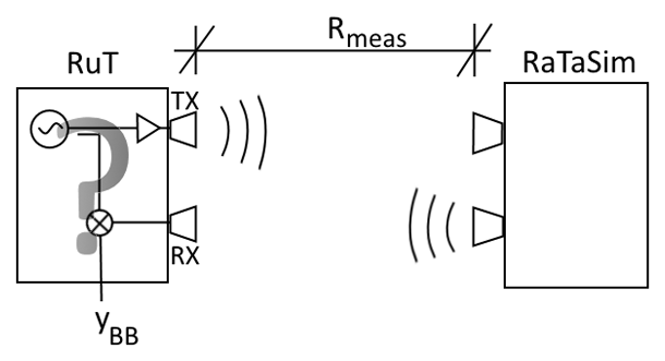
In Fig. 1 the schematic setup for radar target simulation is given. Only continuous-wave (CW) radars (frequency-modulated, frequency shift-keying or classical Doppler CW) will be investigated here. On the right side the radar under test (RuT) including an internal signal source (e.g. at 24 GHz), an amplifier, a mixer and RX and TX antennas is shown. At a distance Rmeas the RaTaSim is located. It receives the RuT signal, modifies it and sends it back towards the radar under test. The RuT has a double sideband downconverting mixer. It can also be supposed to have a single sideband mixer (I and Q channel). Let the line between RuT and RaTaSim be defined as x-axis with x=0 at the RuT. The transmit signal from the TX antenna is
assuming that the radar operating frequency ωRuT is firstly not varying over the time but which will be done later. The actual phase φ0 includes the phase at the time t=0. The received signal when reflected back from a real target in the scenery is
The amplitude can be derived by the radar equation which includes the path losses, the radar cross section of the target, atmospheric attenuation and the angle-dependent gain of the RX and TX antennas. The calculation of B is of no interest here. is the time-of-flight of the signal which travels twice the distance RTarget with the speed of light c0.
Converting down the transmit signal with the receive signal and a subsequent low-pass filtering with fLP indicating the low-pass filtering function yields the baseband (BB) output signal of the RuT

It is obvious that when ωRuT is changing linearly (linear FMCW-ramp) the output of RuT is oscillating for a non-moving target. The further away the target, the faster the oscillation of the RX signal becomes due to the linear FMCW ramp. A classical Fourier transform allows separation of different targets at different ranges.
A radar target simulator must simulate the same wave propagation so that the output of the radar yields the same signal as described in Eq. (3).
Let us assume that the RaTaSim consists of an internal RF source which is very stable at frequency ωRTS (e.g. PLL-locked). Figure 2 shows the schematical setup of the RaTaSim. The frequency of the internal source ωRTS is not in the band of interest (e.g. 23.8 GHz for the 24 GHz ISM band). The source signal could be given by
The source signal has not to match the transmit signal frequency of the RuT. The receive signal of the RaTaSim is
being Cint and CRX the amplitude of the internal source signal of the RaTaSim and the amplitude of the receive signal. Rmeas is the physical distance between RuT and RaTaSim as indicated in Fig. 1.
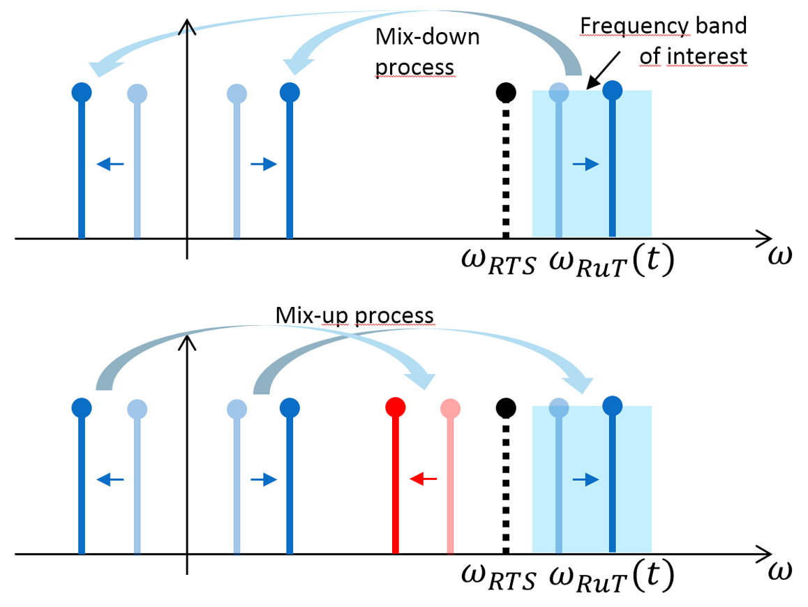
Both signals are mixed via a double sideband mixer yielding only a real baseband signal after low-pass filtering. This signal is of “low” frequency somewhere between DC and several GHz. The complete signal is delayed by a “low-frequency” baseband delay line. The delayed signal is again upconverted over a double sideband mixer with the same internal source signal. The internal signal is supposed to be shifted due to further electronic delays Δtint.. A diagram about the derived frequencies and their relative location could be found in Fig. 3.
The following equation gives the mathematical description of the up conversion.
It is obvious that the right frequency point has the original receive frequency which can be represented as
The frequency of the left frequency point is
which is the mirror frequency of ωRuT mirrored at ωRTS. If the RaTaSim source frequency is located out of the band (mostly below the band, e.g. at 23.8 GHz) and ωRuT is located within the band the mirror frequency will be below ωRTS and located out of the band, too. It is possible to transmit the complete frequency composition towards the RuT. When converting down the left frequency point in the radar system, a difference frequency of approximately 2Δω is occuring (in our example at least 400 MHz). This will be filtered out by the RuT. In Engelhardt et al. (2016) it is proposed to filter out the mirror frequency. Thus, it is important to keep a certain offset between the internal RaTaSim frequency and the lower edge of the frequency band. When using narrowband patch arrays, the left-side frequency point is filtered out by the antenna itself.
For the further development we neglect this frequency component. The upconverted signal is again transmitted by the TX antenna of the RaTaSim and received by the RuT, the delay time TDelay can be represented as an equivalent distance ΔR.
The receive signal at the radar-under-test is as follows
Converting down in the RuT yields the following signal
Bsim and Csim are the amplitudes of the receive and baseband signal due to radar target simulation and should be equivalent to the amplitudes B and C in Eqs. (2) and (3). Compared to the baseband signal of a real target described in Eq. (3), the simulated distance Rsim corresponds to the real target's distance RTarget. But in addition there is an additional phase shift . The second part is not changing while ωRTS is constant. The constant phase can be interpreted as a phase shift at the reflection plane of a target. In the case of changing ωRTS a variable error is occuring.
Furthermore the first part ωRTS⋅TDelay is including an additional constant phase shift when both factors are constant. When TDelay is changing, which is important for dynamic simulations, a erroneous Doppler shift is occuring in addition to the real Doppler with
It can be suggested that this erroneous Doppler can be compensated when changing ωRTS in the manner that with changing ΔR the phase shift stays constant. This method has limitations. On the one side the RaTaSim signal source is limited in frequency range and furthermore a simulation of multiple targets will not be possible when adjusting ωRTS for one target. Thus the radar target simulation with out-of-band source is limited and simulations allowing Range-Doppler processing in the RuT are not possible.
The commercial simulators presented in Diewald and Culotta-Lopez (2017) are mostly not low-cost. Especially the simulators from dedicated manufacturers of RF-measurement technologies like ROHDE & SCHWARZ (Rohde & Schwarz, 2018), KEYSIGHT (Keysight, 2018), ANRITSU (Abou-Jaoude and Grace, 2000) and NATIONAL INSTRUMENTS (Everly, 2016) are based on their RF-measurement technology which is of high cost starting from several EUR 100 000. The simulators coming from other manufacturers like PERISENS (Engelhardt et al., 2016), SMART MICROWAVE SYSTEMS (SMS, 2018) and RFBEAM (RFbeam, 2018) have non-variable ranges for only one single target or dynamic ranges with high step sizes for few targets. For the latter the targets are “jumping” in the range domain, while the Doppler is simulated by an additional Doppler shift which is not physical.
In this section a radar target simulator with an in-the-band-source is presented (Diewald and Leuck, 2015). For low baseband frequencies and thus a low-cost implementation of the Radar Target Simulator, the RaTaSim source signal frequency is now located in the middle of the band of interest (e.g. at 24.125 GHz for the ISM band). Due to the low frequency of the baseband signals these can be digitized and delayed in a logic unit.
The formulas as derived in the section before can still be used. But due to the location of ωRTS exactly in the middle of the band the mirror frequency (formerly known as ωleft) is located in the band, too. It will be filtered out when the distance between both frequencies is higher than the output low-pass frequency of the RuT. Nevertheless disturbances are arising when both frequencies are close together which will occur in each frequency ramp. It can be supposed that with the actual hardware setup the simulation of artificial radar targets is not possible due to the mirror frequency caused by double sideband mixers. The setup is modified in the following manner: single sideband mixers for down- and upconversion are used. Due to these mixers two signals are available in the baseband, the in-phase (I) and the quadrature (Q) signal.
The Q-signal is shifted by 90∘ to the I-signal. Mixing this signal not with Eq. (4) but with a signal shifted by 90∘ yields a RF signal which is quite similar to Eq. (6) except the mirror frequency shifted by 180∘. Thus when adding both signals only the original frequency component ωRuT is remaining.
The complete mixture process can now be considered in the complex domain. The real RaTaSim receive signal (Eq. 5) can be described in complex form
Mixing Eq. (14) with the complex internal signal (compare Eq. 5)
allows to distinguish the I-channel by the real part and the Q-channel by the imaginary part.
Converting up with the conjugate-complex internal RaTaSim signal (but with negative sign in the exponential function)
allows the reconstruction of the original receive signal by the real part
which is the same equation as Eq. (13) neglecting the artificial delay and an internal electronic time delay. It will be supposed that the complex signal is delayed by TDelay before converting up which yields a phase shift over frequency in the complex domain. The complete mixing process including this additional delay can be described as
where the receive signal is directly represented as complex signal (in order to neglect the filtering in the calculation)
As the delay will later be implemented in the baseband the delay term needs to be separated into two terms.
The complex signal is delayed by the time TDelay. The two physical signals I and Q can be interpreted as complex signal but with additional phase shift.
This derivation shows that in order to delay the radar signal in the RF domain without an additional phase shift as it occurs by converting down with a double sideband mixer (as in Sect. 2) the complex signal must be multiplicated with in order to suppress the additional phase shift. Thus the usage of an I∕Q mixer for radar target simulation is one of the major advantages. This yields for the real signals which are upconverted:
An in-the-band source has the advantage of dividing the band into two parts of same bandwidth size. In the baseband channels only signals from up to (with Δf being the bandwidth) are arising. This allows lower sampling rates for analog-digital-conversion. For example the system presented in Diewald (2017) operates in the 24 GHz ISM band with a bandwidth of 250 MHz. The system uses double sideband converting mixers with LO frequency located in the middle of the band which yields a I∕Q baseband signal with 125 MHz bandwidth each. Figure 4 shows the complete schematic of the radar target simulator.
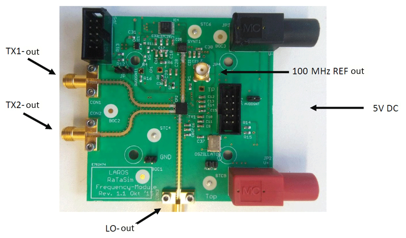
All RF- and baseband electronics are developed in our institution in a modular approach by using semiconductor components (e.g. I∕Q mixers, VCO, LNA, PLL, etc.) which are based on radar technology from known semiconductor manufacturers producing in the radar frequency range. For example, the internal LO signal is generated by a 24 GHz signal source based on the Analog Devices ADF5901 radar transmitter IC (Steins et al., 2016) which is shown in Fig. 5.
All RF components are designed separately on a four-layer PCB with ROGERS RO4835 top and bottom layer with a FR4 core material and connected by Rosenberger 02K243 connectors. The complete RaTaSim system is implemented in a modular way by low-noise amplifiers (LNA), the variable gain amplifier (VGA), the single sideband mixers including the power divider and the 24 GHz LO signal source which are connected to each other corresponding to the schematic given in Fig. 4.
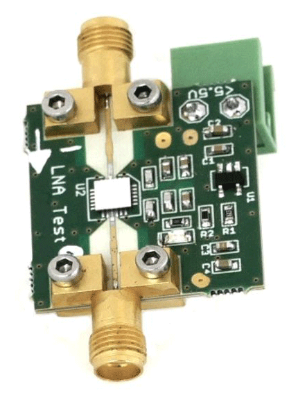
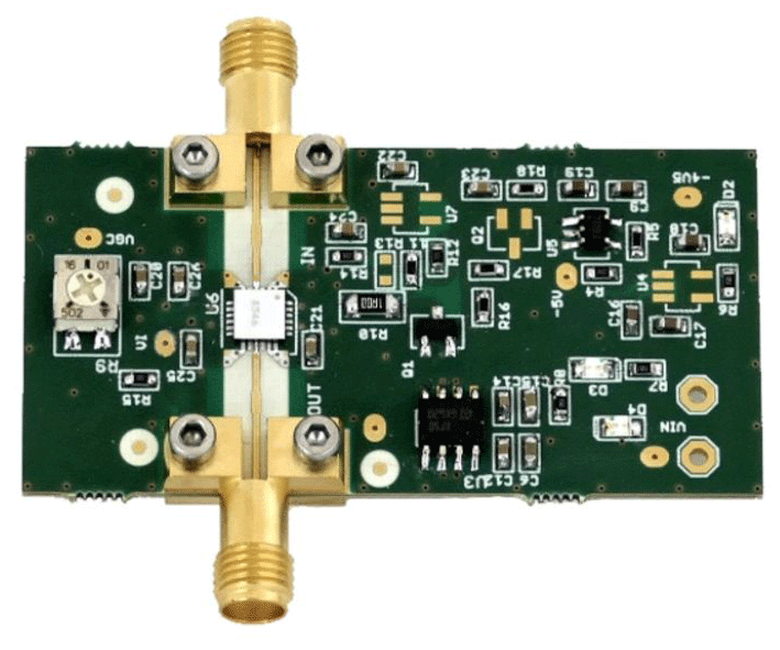
The low-noise amplifier is based on an Analog Devices (formerly Hittite) HMC751 chip which has a frequency range from 20.0 to 28.0 GHz with a gain of approx. 25–26 dB. The power supply voltage level is 4 V. The low-noise amplifier module is shown in Fig. 6.
The variable gain amplifier has a programmable gain between 3 and 16 dB (maximum power of 24 dBm) between 20 and 28 GHz in steps of 1 dB. The used Analog Devices HMC997 chip requires a supply voltage of 5 V and is shown in Fig. 7.
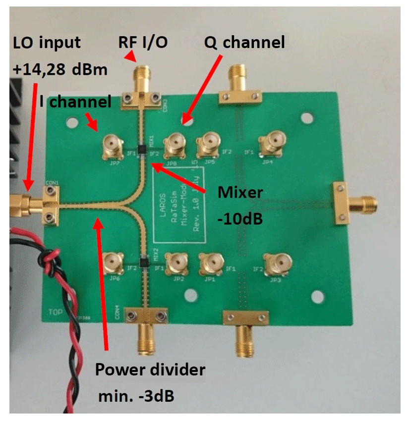
Finally the Analog Devices HMC1063LP3E chip is used as passive single sideband mixer for down- and up-mixing. The I∕Q baseband signals are connected by top-mounted SMA connectors which are shown in Fig. 8. Further passive components are the power dividers developed for 24.125 GHz as center frequency and the six-patch traveling wave antenna (TWA) arrays. The TWA array has a gain of 13.8 dBi, an opening angle (−3 dB) of 19.1∘ and a sidelobe suppression of −12.1 dB. A radiation pattern and the antenna layout is shown in Fig. 9.
Two orthogonal polarisations of the RuT are processed in parallel. This allows the considerations of all polarisation types (linearly and circularly polarized). In contrast to the most RaTaSim systems on the market the antennas are realized in patch antenna technology with a sufficient high isolation between RX and TX channel instead of expensive horn antennas. The complete demonstrator is shown in Fig. 10 where the receive and transmit patch antenna arrays for each polarisation are visible.

Due to the progress in the semiconductor technology the digitization of the baseband signal and the digital implementation of the delay with a fast FPGA offers much flexible processing. The delay is realized by a “virtual” transmission line based on a FIR approach on a Xilinx Kintex-7 KC705 FPGA which allows low-latency processing of the digital data. The analog-digital conversion and the digital-analog conversion must be of high sampling rates, of high resolution and of low-latency, too, which is realized by a 4DSP FPGA Mezzanine Cards FMC151. The additional inaccurate Doppler shift which is caused by the delay in the baseband can be corrected in the FPGA due to the representation of the wave as complex value. The step-size of the radar targets will be in the sub-mm range which allows inherently the modeling of the Doppler effect which has been shown in Diewald (2014).
A simple shift register with programmable taps can be used for this purpose. According the Shannon sampling theorem a minimum sampling rate of 250 MSPS is needed for operation which is the clock frequency of the shift register simultaneously. With 250 MSPS the digital delay line has a minimal resolution of ToF_min=4 ns resulting in range step size of
The digital concept allows a very efficient realization of ranges from 0 m to larger than 300 m with a step resolution of 60 cm. The implementation in VHDL is very easy by using an IP-Core for shift-RAM. For just simulating ranges this would be a satisfactory implementation. For some applications it is necessary to achieve a much finer range or position resolution and also the Doppler effect which occurs for moving targets. This problem can only be solved by a drastic increase of the sample rate and the massively increasing usage of resources or by the use of an interpolation filter where the latter solution is chosen. The interpolation filter is based on a FIR filter topology with coefficients based on the sinc-function . With delay steps which are just multiples of the inverse of the sampling frequency, one single coefficient is sufficient to generate a time-shifted signal, all other coefficients are zero according to the zeros of the sinc function. This implementation lets the target range change in steps of 60 cm. A shift of a signal in time domain yields an additional linear phase shift in the frequency domain.
The product between the Fourier transform of the non-shifted signal and the additional linear phase shift can be interpreted as a classical filtering. The filter function for the FIR filtering could be easily found by an inverse FFT of the exponential function to the discrete time domain. By this implementation there are two things to consider:
-
generally the impulse response of a rectangular window (which is the sinc-function) is infinitely long, but only a filter with finite number of coefficients can be realized for FIR filtering;
-
the filter is non-causal.
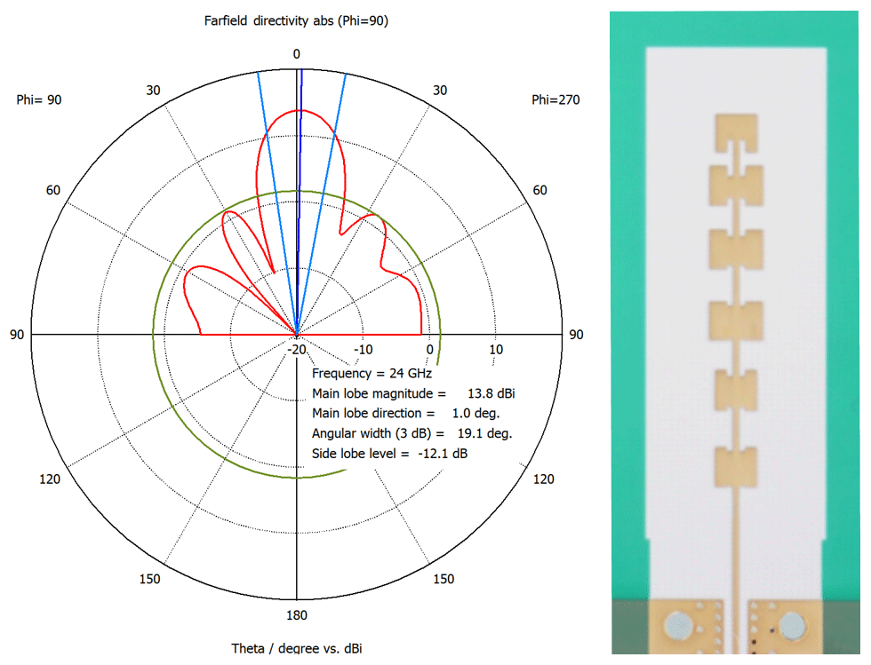
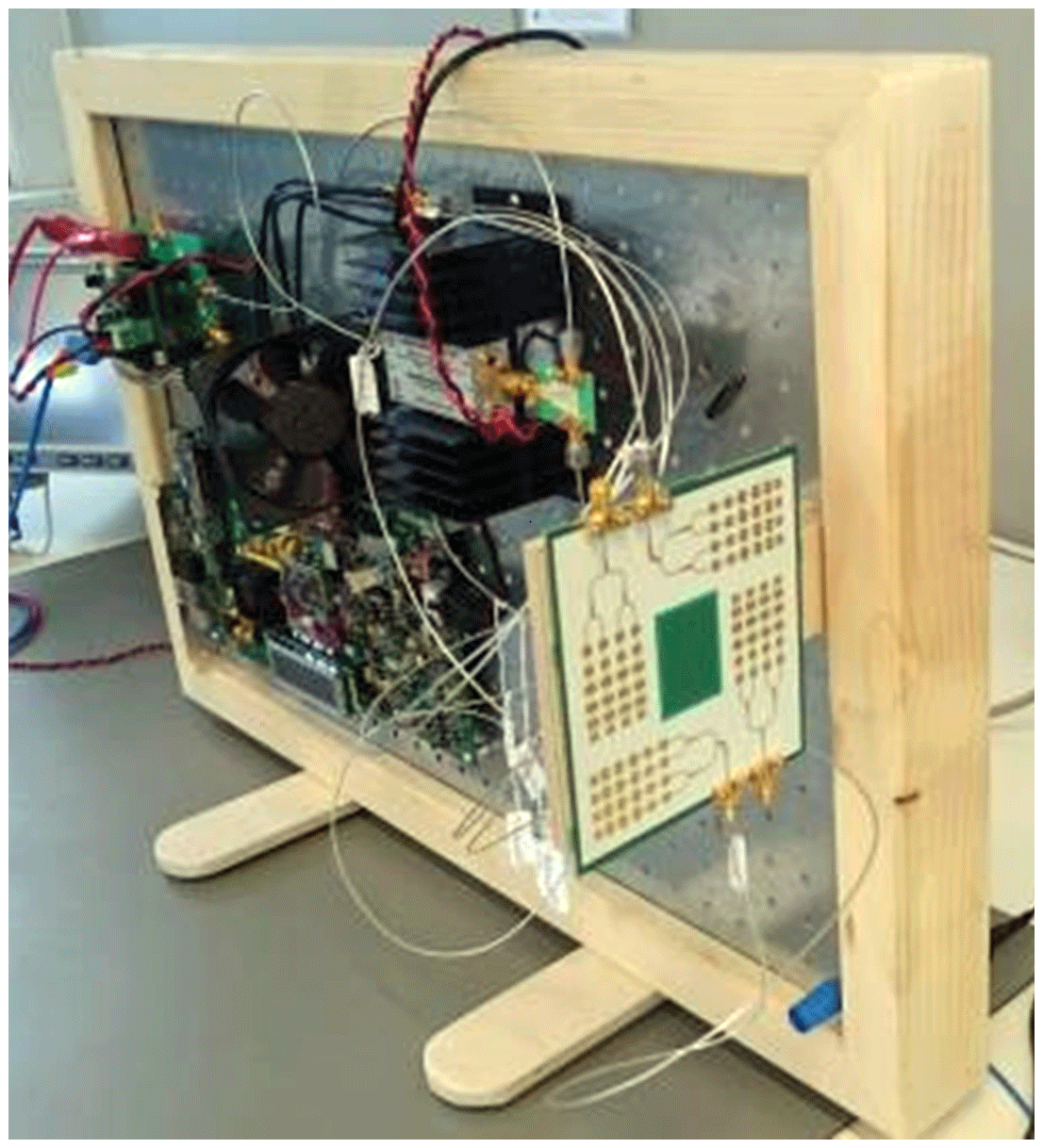
Figure 10Modular 24 GHz RF circuitry with digital electronics (FPGA and ADC/DAC-board) on a wooden frame.
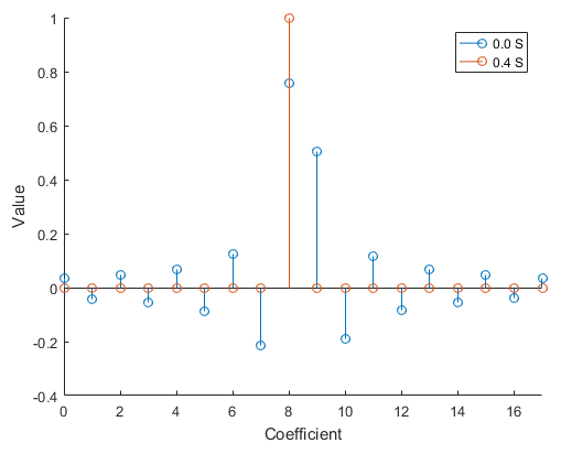
The inverse FFT of the limited bandwidth of 250 MHz will result in a discretization with a time step of 4 ns which corresponds to the 60 cm propagation path in radar applications. The number of filter coefficients is dependent from the number of elements of the exponential function. The number of elements should cover the Shannon theorem, thus the phase shift between adjacent points in the frequency domain is not greater than 180∘. Figure 11 shows the coefficients for a non-shifted signal and a signal shifted by 1.6 ns which is a shift of 0.4 samples.
For large distances the number of points could become quite high. For this reason, and the limited number of existing hardware multipliers in the FPGA, the delay line has been split. A large FIFO shift register generates the coarse delay of 0–300 m with 60 cm step resolution and this is appended to the interpolation filter which has the only task to produce a fine delay between 2 sampling points. The acausality can simply be bypassed by pre-sampling, which of course has the disadvantage that the minimally simulated distance of the radar target simulator is increased. So there has to be a trade-off between the number of coefficients and the directly related signal quality as well as the increasing latency and the resource consumption. A filter length of NFIR_taps=18 taps seems to be satisfactory, as well as 16 bit data resolution and 18 bit coefficient resolution is applied. By using the filter with these parameters in the radar target simulator, the minimum target distance which can be simulated increases by m.
The filter coefficients are calculated with Matlab, the so-called coefficient files were integrated directly with the development environment and stored in the Block-RAM of the FPGA. Due to the fixed structure of the hardware RAM blocks, 2048 different variants can be interpolated, which theoretically corresponds to a distance resolution of 300 µm. Such a fine resolution generates a Doppler shift automatically which has been already proven in Diewald and Culotta-Lopez (2017). The practical implementation in VHDL for the design to operate with the high sample rate is very problematic. In this case it is absolutely necessary to create a pipelined filter structure on the FPGA. The interpolation filter is programmed onto the FPGA including a phase rotation which corrects for the wrong Doppler shift when the simulated target is moving.
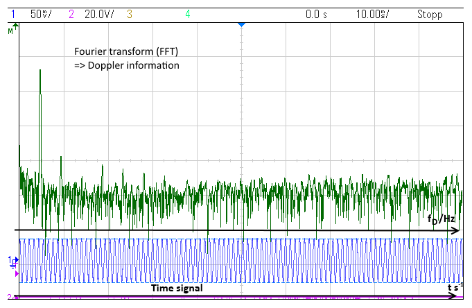
The complete demonstrator is tested with a 24 GHz laboratory radar (RuT) based on the ADF5901 and ADF5904 ICs from Analog Devices. The baseband output of the the RuT has been connected to a Keysight MSOX2014A Mixed Signal Oscilloscope with a Fourier transform option. The first measurement was a classical CW-measurement with a frequency of 24.00 GHz and the simulated target is moving with 11.875 m s−1. An oscilloscope screenshot of the measurement is shown in Fig. 12.
The baseband output is measured and the Doppler frequency is determined by Fourier transform with 950 Hz which is equivalent to the analytical result of the following equation
where c0 is the speed of light, vD the target's speed and f0 the CW-frequency. Due to a purely real baseband signal the direction of motion could not be detected. But for a RuT including I∕Q baseband outputs this would be possible with the radar target simulator presented here. For the next measurement the operation mode of the RuT is changed to a triangular FMCW mode with upward and downward ramps with a ramp repetition rate of 100 s−1 over 250 MHz. This means that the ramp slope for one ramp is MHz/5 ms. The trigger input of the oscilloscope is set to the beginning of the upward ramp. The storage time also covers the downward ramp. The simulated target is set to a distance of 100 m and moving towards the RuT at a velocity of 11.875 m s−1. The baseband signal and the related Fourier transform are plotted in Fig. 13. The screenshot was taken at a range distance of currently 53.1 m.
The rough baseband signal (yellow) is Fourier transformed for which two peaks are observable. The frequency of the first peak is 7900 Hz while the frequency of the second peak is 9800 Hz. The mean value of both frequencies is fmean=8850 Hz.
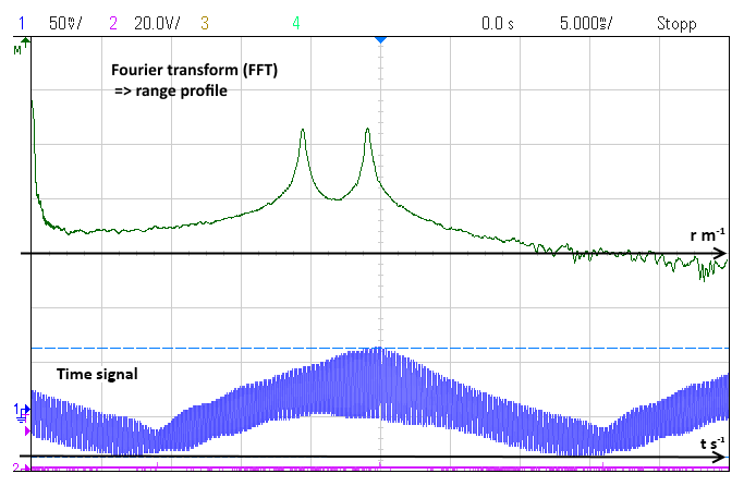
With the formula (Skolnik, 2008)
the measurement shows that the range simulation is correct. The difference between the frequencies is 1900 Hz. The formula to calculate the Doppler shift from a triangular measurement (Skolnik, 2008) is
In addition it is proven that the Doppler simulation is correct by conventional range simulation with fine discretization and Doppler correction.
In this paper a low-cost implementation of a radar target simulator has been presented. Starting with an introduction into radar target simulation, an overview was given shortly. Afterwards the theoretical foundations of radar target simulations were given in a mathematical way with the focus on both double and single sideband mixers. The generated frequencies and their location inside and outside of the band of interest were investigated. Out of that investigation, a concept for a complex-valued transmission line modeling with an I∕Q mixer topology has been presented. This approach allows the inherent Doppler simulation by a correction of the phase information (rotation in the complex domain) when the targets are moving. A demonstrator has been installed that is based on a modular approach in order to prove the simulation concept. The implementation of a fine discretized range simulation by FIR approach has been presented which allows the inherent Doppler simulation. The range and phase shifting has been realized by a FIR filter structure in a FPGA with fast-sampling ADCs and DACs. The digital electronics allows a sampling rate of 250 MSPS which is sufficient for the down-converted signal of the 24 GHz ISM band when mixed down with an “in-the-band” local oscillator source.
Due to transformation of a shifted filter function from the frequency domain to the time domain, the finite number of filter coefficients for the FIR filter have been determined. In order to keep resources, the digital delay line was split into two segments. The first delay segment allows for rough delay steps with a size of 60 cm. The second delay module enables a very fine discretization of the range. This manner permits a very low-cost implementation of the radar target simulator in the 24 GHz ISM band. A correct Doppler and range evaluation showed that the concept is valid and could be used for series-development of the hardware. In a next step, a new design of the RF and baseband electronics will be developed which will bring any modular components together, allowing an integration into a housing.
No data sets were used in this article. The FPGA code is not public and are only available from the corresponding author upon request.
ARD conceived of the present idea and the theory. ARD supervise the project. MS put the complete electronics into operation and implemented the hardware description in VHDL. SM designed the RF-modules and put these into operation.
The authors declare that they have no conflict of interest.
This article is part of the special issue “Kleinheubacher Berichte 2017”. It is a result of the Kleinheubacher Tagung 2017, Miltenberg, Germany, 25–27 September 2017.
The author would like to thank ANALOG DEVICES, especially Rudolf Wihl, Dirk Legens,
Bernd Krätzig and Christian Eisenschmidt for the kind support.
Edited by: Madhu Chandra
Reviewed by: Andreas Danklmayer and one anonymous referee
Abou-Jaoude, R. and Grace, M.: Test systems for automotive radar, VTC2000-Spring, in: 2000 IEEE 51st Vehicular Technology Conference Proceedings, vol. 1, Tokyo, 492–495, 2000. a
Diewald, A. R.: Doppler analysis and modeling of complex motions in layered media, in: 44th European Microwave Conference (EuMC) 2014, 6-9 October 2014, Rome, 471–474, 2014. a
Diewald, A. R.: A Low-Cost Radar Target Simulator, in: Kleinheubacher Tagung 2017, Miltenberg, 2017. a
Diewald, A. R. and Culotta-Lopez, C.: Concepts for Radar Target Simulation, in: The Loughborough Antennas and Propagation Conference, 13 November 2017, available at: https://www.hochschule-trier.de/fileadmin/groups/127/template/Publications/RaTaSim_Concept_-_LAPC.pdf (last access: 15 October 2018), 2017. a, b, c
Diewald, A. and Leuck, S.: Abstandsimulierendes Radartarget, Deutsches Marken- und Patentamt, DE 10 2015 121 297, application date: 8 December 2015. a
Diewald, A. R., Landwehr, J., Tatarinov, D., Di Mario Cola, P., Watgen, C., Mica, C., Lu-Dac, M., Larsen, P., Gomez, O., and Goniva, T.: RF-based child occupation detection in the vehicle interior, in: 17th International Radar Symposium (IRS), Krakow, 2016. a
Engelhardt, M., Pfeiffer, F., and Biebl, E.: A high bandwidth radar target simulator for automotive radar sensors, in: 2016 European Radar Conference (EuRAD), London, UK, 245–248, 2016. a, b
Eyerly, D.: TS10105 —Testing Automotive Radar Sensors With the NI Active Target Simulator and a LabVIEW-Based Scene Editor, in: National Instruments Week, 3–4 August 2016, Austin, Texas, 2016. a
Keysight Technologies: E8707A Radar Target Simulator 76 GHz to 77 GHz, available at: http://literature.cdn.keysight.com/litweb/pdf/5992-1648EN.pdf, last access: 26 November 2018. a
RFbeam: K-DT1 Radar Doppler Target, available at: http://rfbeam.ch/files/products/32/downloads/ProductBrief_K-DT1.pdf, last access: 26 November 2018. a
Rohde & Schwarz: ARTS9510 Automotive Radar Simulators, available at: https://cdn.rohde-schwarz.com/pws/dl_downloads/dl_common_library/dl_brochures_and_datasheets/pdf_1/Flyer_ARTS9510C.pdf, last access: 26 November 2018. a
Skolnik, M. I.: Radar Handbook, 3rd Edn., McGraw-Hill Education, New York City, USA, 2008. a, b
SMS – Smart Microwave Sensors: KTSDG-02, available at: http://www.smartmicrogroup.com/fileadmin/user_upload/Documents/Automotive/KTSDG-02xxxx_Datasheet.pdf, last access: 26 November 2018. a
Steins, M., Leuck, S., and Diewald, A.: Universal Programmable Low Cost Signal Source for 24 GHz ISM Band, in: The Loughborough Antennas and Propagation Conference (LAPC), 12 November 2016, Loughborough, 2016. a