 | 19 Sep 2019
Towards a Spectral Method of Moments using Computer Aided Design
Stefan Kurz
Sebastian Schöps
We present first numerical examples of how the framework of isogeometric boundary element methods, in the context of electromagnetism also known as method of moments, can be used to achieve higher accuracies by elevation of the degree of basis functions. Our numerical examples demonstrate the computation of the electric field in the exterior domain.
- Article
(2101 KB) - Full-text XML
- BibTeX
- EndNote


Spectral methods, cf. Trefethen (2000), are classes of methods for solving differential equations, closely related to classical element based methods. They share the same idea: The approximation of the solution through a series of basis functions. While classical methods choose to refine a mesh, and with this to further localise the support of each individual basis function, spectral methods employ global basis functions to approximate the solution of the problem. Since such a global basis is not always readily available, quite often any finite and boundary element method which relies solely on p-refinement, i.e., the increase of the degree of the local without mesh (h-) refinement, is referred to as a spectral element method.
In engineering applications, spectral element methods are rarely considered; the reason simply being that to fully enjoy their convergence properties, meshes with curved elements of increasing orders must be generated. This poses challenges to mesh generation and pre-processing. In contrast, classical h-refinement based mesh generators are well understood. However, with the introduction of isogeometric analysis by Hughes et al. (2005) the problem of efficient mesh generation can be avoided by the use of exact geometry mappings, allowing computations directly on CAD-generated objects.
In this document, we present numerical experiments which showcase how the isogeometric framework can be used to obtain an implementation of a spectral boundary element method. We demonstrate the implementation by the solution of electromagnetic scattering problems through p-refinement. For this, we employ a solution strategy via the electric field integral equation (Buffa and Hiptmair, 2003), which is also referred to as method of moments (MOM), and an isogeometric boundary element framework (Dölz et al., 2018b). We essentially employ p-refinement to a patchwise polynomial basis, in our case based on Bernstein polynomials. Other variants of spectral MOM have already been studied, eg. by Benoit et al. (1992) or Di Ruscio et al. (2014).
The organisation of the paper is straight forward. We first introduce basic notions of the electric field integral equation, and our p-refinement based discretization scheme, built on top of the framework of isogeometric analysis. Afterwards, we comment on the matrix assembly, followed by a discussion of our numerical examples.
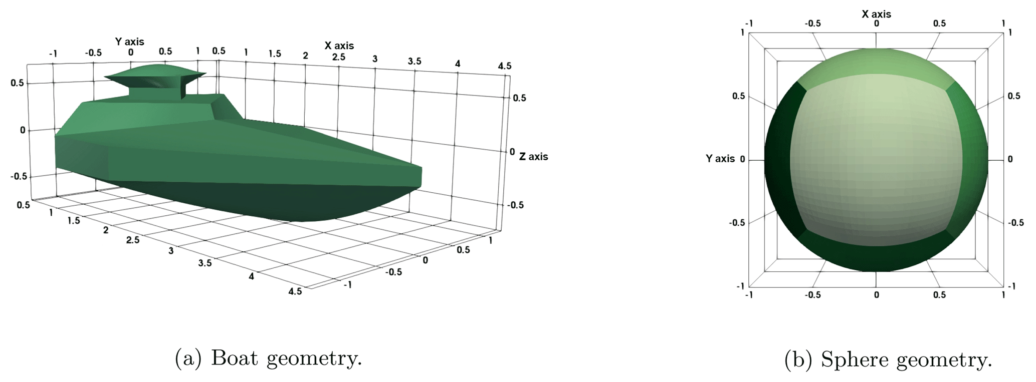
Figure 1Visualisations of the geometries. The maximum diameter of the boat is smaller than 4.5, the sphere is of radius 1.
We consider the scattering of an electromagnetic wave under the assumption of constant material coefficients μ and ϵ in Ωc, i.e., the surroundings of a scatterer Ω, PEC boundary condition on and the Silver-Müller radiation condition. Prescribing an incident wave g we arrive at
with wave number Herein, n denotes the outward unit normal of Γ. Under these conditions, there exists a surface current j such that the scattered field can be represented by the electric field integral equation (EFIE), given by
with
for all Herein, denotes the Green's function given by cf. Buffa and Hiptmair (2003) for details.
In a continuous setting, this can be recast as the variational problem of finding an unknown surface current j in the trace of the space H(curl,Ω), such that
holds for all test functions ξ in the same space. The corresponding trace space is often denoted by and requires a divergence-conforming discretisation.
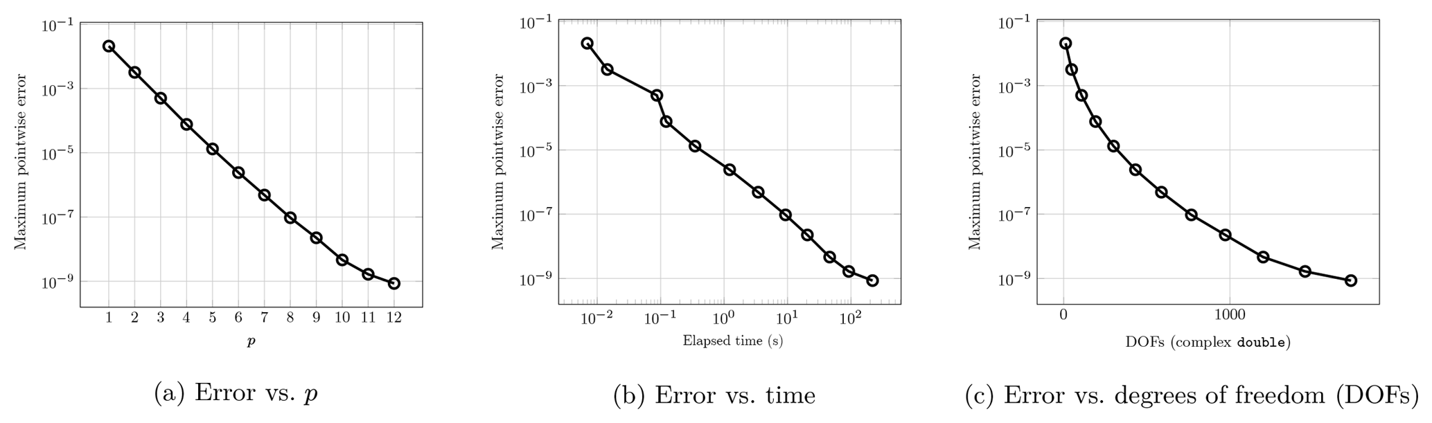
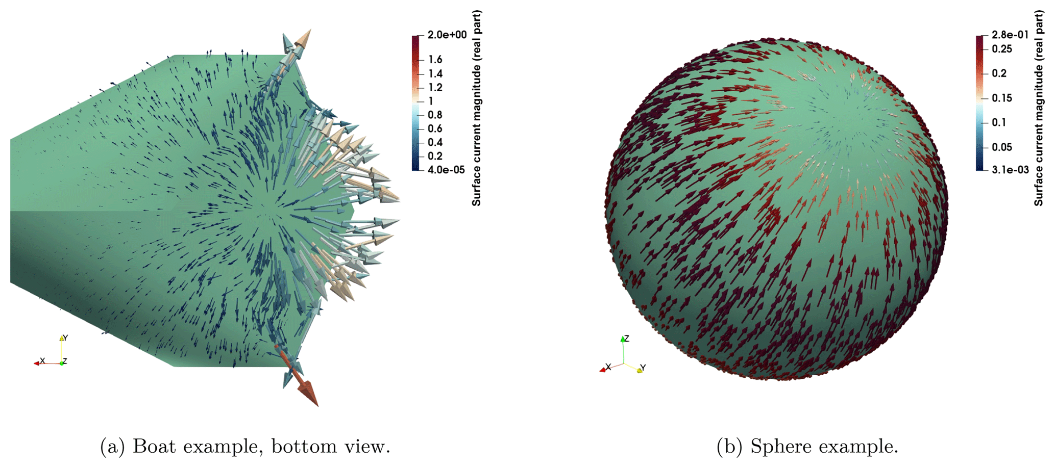
Figure 3Numerical examples on the unit sphere. Wave number κ=1. The error refers to the maximum error obtained by comparing the values of the analytical solution with the field values through evaluation of Eq. (2) on a selection of 10 000 points on a sphere of radius 2 around the origin. Computed on a desktop PC with 16 GB RAM and an Intel i7 8700k processor.
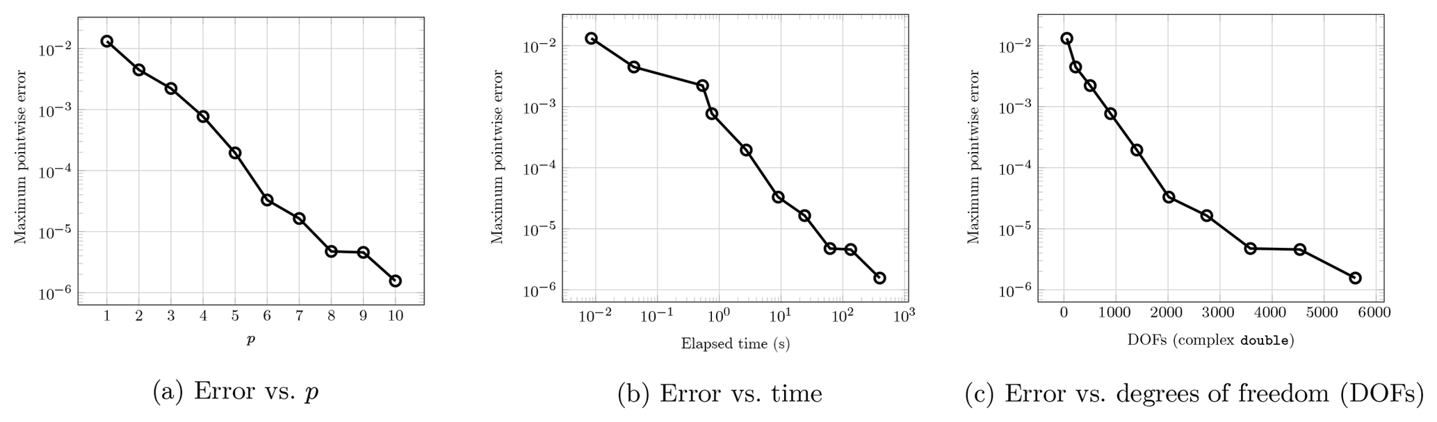
Figure 4Numerical examples for the ship geometry as presented in Fig. 1a. Highest p generates a discretisation with 5600 complex-valued degrees of freedom. Wave number κ=1. The error refers to the maximum error obtained by comparing the values of the analytical solution with the field values through evaluation of Eq. (2) on a selection of 10 000 points on a sphere of radius 6 around the origin. Computed on a desktop PC with 16 GB RAM and an Intel i7 8700k processor.
To solve the electric wave equation via a boundary element approach, the unknown is reduced to a vector field on Γ, often discretised by divergence-conforming elements. Implementations of such and related numerical schemes are, among others, given by Hiptmair and Kielhorn (2012), Tzoulis and Eibert (2005), or Weggler (2011). We utilise an approach based on the framework of isogeometric analysis, dealing with the special case where the B-spline basis reduces to the set of Bernstein polynomials, for order p≥0 given by
To apply p-refinement, one needs sufficiently smooth (patchwise) geometry mappings, since otherwise they limit the order of ansatz functions which can be applied effectively. Thus, we choose geometry mappings given by mappings from the unit square to parts of the geometry Γj parametrized as tensor product mappings of rational Bernstein polynomials. Such representations can be easily extracted from NURBS (non uniform rational B-Spline) parametrisation through Bézier extraction (Borden et al., 2011).
Following Buffa et al. (2011), a suitable discretisation of the trace spaces on so-called multipatch domains , i.e., elements in the context of spectral element methods, is provided in Buffa et al. (2018). By tensor product construction one constructs discrete spaces that are conforming w.r.t. the differential operators. As an example, if Sp denotes the Bernstein polynomials of order p≥1 on (0,1), one finds that
holds. This way, using the NURBS geometry mappings induced by the CAD geometries to seamlessly map between (0,1)2 and patches Γj⊆Γ, one can define a conforming discretisation of the entire de Rham complex
as well as its trace spaces
which is required for the analysis of boundary element methods. In the case of the divergence-conforming space, one must require additional normal continuity of the vector field across patch interfaces. This can be achieved through identification of the corresponding degrees of freedom (DOFs) with one another. We denote the discretisation on the boundary defined Buffa et al. (2018) by
For these spaces, it is possible to show existence, uniqueness, and quasi-optimality of the solution (Dölz et al., 2018b). The discrete problem to Eq. (4) is that of finding a discrete surface current such that
holds for all test functions The coefficients to represent , where the ξh,j denote the basis functions of can be obtained in form of the vector c given by the solution to the linear system Ac=r, where A and r can be assembled in direct analogy to Eq. (8).
We apply a modified version of the superspace approach as used by e.g. Dölz et al. (2018a) to construct the dense system matrix A resulting from Eq. (4) via the representation
where A† is the dense system matrix w.r.t an elementwise polynomial, globally discontinuous basis, and P is the superspace matrix assembling the divergence-conforming basis. Herein, each matrix is sparse, including only the interaction of the local basis on element i with that of element j. This way, the small dense system A is assembled without the need to store A† as a whole. In the special case of only p-refinement, the matrix P incorporates only linear combinations necessary to reduce the degree in one tensor product direction for the construction of , and to achieve normal continuity across patch interfaces. For the solution of the arising linear system, we utilise a partially pivoted LU decomposition of the Eigen linear algebra library (Guennebaud et al., 2010).
To showcase the possibility of obtaining an increased accuracy through (mainly) p-refinement, we present a simple numerical example in analogy to the ones for h-refinement presented by Dölz et al. (2018a).
We excite our model setup by a Hertz-Dipole as defined by Jackson (1998, p. 411) as
with and . The dipole's singularity is placed inside Ω. Away from its singularity, specifically within the exterior domain, the dipole fulfils Eq. (1). Thus, by existence and uniqueness of the solution of the exterior problem Eq. (4), cf. Buffa and Hiptmair (2003), we know that Eq. (8) will approximate the surface current required to represent the field cf. Dölz et al. (2018b). This construction using a prescribed solution is known as a method of manufactured solutions, cf. Oberkampf and Roy (2010, Chap. 6.3).
Summarised, we solve for j in Eq. (8) with an excitation given by Eq. (9). We then evaluate Eq. (2) numerically with the approximated surface current jh whose induced eh(x) yields the numerical solution. By existence and uniqueness eh is an approximation to EDP in the exterior. We compute the error at points x in a set V containing points placed on a sphere enclosing the geometry, see the captions of Figs. 3 or 4 for details.
As a first example, we choose the example of a unit sphere given by 6 patches and define a dipole with as an excitation. Although a boundary element framework has been utilised to solve the problem, no compression was applied to the systems due to their small system size, cf. Fig. 3c.
Thus the condition of the system matters little compared to the case in which compression must be applied.
On the sphere, a stable exponential rate of convergence w.r.t. p is observed. The application of p-refinement reduces the time required for matrix assembly as well as the overall system size, cf. Fig. 3, significantly.
We present another example. As geometry, we choose the boat depicted in Fig. 1 consisting of 28 Bézier patches. Placing the dipole inside with and , i.e., under the “bridge”, we evaluate the electric field around the geometry. For this non-smooth and non-convex geometry, the rate of convergence, as seen in Fig. 4, is not as pronounced as before. Still, one can see an exponential convergence behaviour paired with excellent times to solution.
The adaptation of isogeometric to spectral element methods is straight forward. Through the use of Bézier extraction, one extracts piecewise smooth parametrisations of geometries. Using known constructions from isogeometric analysis, one can define a global, divergence-conforming basis that consists of tensor product Bernstein polynomials, with supports consisting of one patch each, or in the case of functions identified to achieve normal continuity, multiple patches. Application of p-refinement to this basis yields a spectral method of moments, which achieves high accuracies without the need for system compression.
These results are exceptionally promising since the reduced system size makes the application of direct solvers possible, thus circumventing the need for preconditioners, which are still a challenging topic for boundary element methods for electromagnetic problems.
The code basis, as well as the geometries for these computations are available at http://www.bembel.eu/ (last access: 21 May 2019). A fork of the repository ready to recreate the computations can be found at https://github.com/flx-wlf/bembel/tree/ars2019aa/ (last access: 21 May 2019). See also Dölz et al. (2019) (https://doi.org/10.5281/zenodo.2671596).
All authors have jointly carried out research and worked together on the manuscript. The numerical tests have been conducted by the last author. All authors read and approved the final manuscript.
Stefan Kurz is also affiliated as Chief Expert with Robert Bosch GmbH.
This article is part of the special issue “Kleinheubacher Berichte 2018”. It is a result of the Kleinheubacher Tagung 2018, Miltenberg, Germany, 24–26 September 2018.
The work of Felix Wolf is supported by the Excellence Initiative of the German Federal and State Governments and the Graduate School of Computational Engineering at TU Darmstadt.
This research has been supported by the DFG (grant no. SCHO1562/3-1) and the DFG (grant no. KU1553/4-1).
This paper was edited by Thomas Eibert and reviewed by three anonymous referees.
Benoit, C., Royer E., and Poussigue, G.: The spectral moments method, J. Phys. Condens. Matter., 4, 3125–3152, 1992. a
Borden, J., Scott, M. A., Evans, J. A., and Hughes T. J. R.: Isogeometric finite element data structures based on Bézier extraction of NURBS, Int. J. Numer. Meth. Eng., 87, 15–47, 2011. a
Buffa, A. and Hiptmair, R.: Galerkin boundary element methods for electromagnetic scattering, Lect. Notes Comp. Sci., 31, 83–124, 2003. a, b, c
Buffa, A., Rivas, J., Sangalli, G., and Vázquez, R.: Isogeometric discrete differential forms in three dimensions, SIAM J. Numer. Anal., 49, 818–844, 2011. a
Buffa, A., Dölz, J., Kurz, S., Schöps, S., Vázquez, R., and Wolf, F.: Multipatch approximation of the de Rham sequence and its traces in isogeometric analysis, submitted, preprint available: arXiv:1806.01062, 2018. a, b
Di Ruscio, D., Burghignoli, P., Baccarelli, P., Comite, D., and Galli, A.: Spectral Method of Moments for Planar Structures With Azimuthal Symmetry, IEEE T. Antenn. Propag., 62, 2317–2322, https://doi.org/10.1109/TAP.2014.2302831, 2014. a
Dölz, J., Kurz, S., Schöps, S., and Wolf, F.: A Numerical Comparison of an Isogeometric and a Classical Higher-Order Approach to the Electric Field Integral Equation, submitted, preprint available: arXiv:1807.03628, 2018a. a, b
Dölz, J., Kurz, S., Schöps, S., and Wolf, F.: Isogeometric Boundary Elements in Electromagnetism: Rigorous Analysis, Fast Methods, and Examples, submitted, preprint available: arXiv:1807.03097, 2018b. a, b, c
Dölz, J., Harbrecht, H., Kurz, S., Multerer, M., Schöps, S., and Wolf, F.: Bembel v0.9, https://doi.org/10.5281/zenodo.2671596, 2019. a
Guennebaud, G. and Jacob, B.: Eigen v3, available at: http://eigen.tuxfamily.org (last access: 21 May 2019), 2010. a
Hughes, T. J. R., Cottrell, J. A., and Bazilevs Y.: Isogeometric analysis: CAD, finite elements, NURBS, exact geometry and mesh refinement, Comput. Meth. Appl. Mech. Eng., 194, 4135–4195, 2005. a
Jackson, J. D.: Classical Electrodynamics, Wiley and Sons, New York, 3rd edition, 1998. a
Oberkampf, W. L. and Roy, C. J.: Verification and Validation in Scientific Computing, Cambridge University Press, Caimbridge, 2010. a
Trefethen, L. N.: Spectral Methods in MATLAB, SIAM, Philadelphia, 2000. a
Tzoulis, A. and Eibert, T. F.: A Hybrid FEBI-MLFMM-UTD Method for Numerical Solutions of Electromagnetic Problems Including Arbitrarily Shaped and Electrically Large Objects, IEEE T. Antenn. Propag., 53, 3358–3366, 2005. a
Hiptmair, R. and Kielhorn, L.: BETL – A generic boundary element template library, Seminar for Applied Mathematics, ETH Zürich, Rep. no. 36, 2012. a
Weggler, L.: High Order Boundary Element Methods, Dissertation, Universität des Saarlandes, Saarbrücken, 2011. a