Using analog computers in today's largest computational challenges

Analog computers can be revived as a feasible technology platform for low precision, energy efficient and fast computing. We justify this statement by measuring the performance of a modern analog computer and comparing it with that of traditional digital processors. General statements are made about the solution of ordinary and partial differential equations. Computational fluid dynamics are discussed as an example of large scale scientific computing applications. Several models are proposed which demonstrate the benefits of analog and digital-analog hybrid computing.

1 Introduction

Digital computing has transformed many — if not close to all — aspects of industry, humanities and science. Turing completeness allows statements to be made about the computability and decidability of problems and computational power of machines. Digital storage has undergone numerous technological advances and is available in increasingly vast amounts. Nevertheless, contemporary digital computing is possibly not the last word in computing, despite its dominance in the consumer market for the last 40+ years.

Fundamental research about non-traditional (also referred to as unconventional or exotic) computing is taking place in material sciences, chemistry but also in more exotic branches such as biology and life sciences. Amongst others, beyond-Turing computing (Siegelmann, 1995), natural computing (Calude et al., 1999), neuromorphic computing (Schuman et al., 2017; Ziegler, 2020) or quantum computing (Zhou et al., 2020; Georgescu et al., 2014; Kendon et al., 2010) are fields of active investigation. Being fundamental research at heart, these disciplines come with technological challenges. For instance, computing with DNA still requires the use of large scale laboratory equipment and machinery (Deaton et al., 1998). Currently, not only the low-temperature laboratory conditions but also the necessary error correction schemes challenge practical quantum computers (Wilhelm et al., 2017). This currently negates any practical advantage over silicon based digital computing. Furthermore, all of these alternative (or exotic) computer architectures share the characteristic that they are fundamentally non-portable. This means they will have to be located at large facilities and dedicated special-purpose computing centers for a long time, if not forever. This is not necessarily a practical drawback, since the internet allows for delocalization of systems.

In contrast to this, silicon based electronic analog computing is a technology with a rich history, which operates in a normal workplace environment (non-laboratory conditions;  Ulmann, 2020). Digital computers overtook their analog counterparts in the last century, primarily due to their ever-increasing digital clock speeds and their flexibility that comes from their algorithmic approach and the possibility of using these machines in a time-shared environment. However, today Moore's law is coming to a hard stop and processor clock speeds have not significantly increased in the past decade. Manycore architectures and vectorization come with their own share of problems, given their fundamental limits as described, for instance, by Amdahl's law (Rodgers, 1985). GPGPUs and specialized digital computing chips concentrate on vectorized, and even data flow-oriented programming paradigms but are still limited by parasitic capacitances which determine the maximum possible clock frequency and provide a noticeable energy barrier.

Thanks to their properties, analog computers have attracted the interest of many research groups. For surveys of theory and applications, see for instance Bournez and Pouly (2021) or the works of MacLennan (2004, 2012, 2019). In this paper, we study the usability of analog computers for applications in science. The fundamental properties of analog computers are low power requirements, low resolution computation and intrinsic parallelism. Two very different uses cases/scenarios can be identified: High performance computing (HPC) and low energy portable computing. The energy and computational demands for both scenarios are diametrically-opposed and this paper is primarily focused on HPC.

The paper is structured as follows: In Sect. 2, we review the general assumptions about digital and analog computing. In Sect. 3, small scale benchmark results are presented for a simple ordinary differential equation. In Sect. 4, a typical partial differential equation is considered as an example for a large scale problem. Spatial discretization effects and computer architecture design choices are discussed. Finally, Sect. 5 summarizes the findings.

2 A Simple (Linear) Model for Comparing Analog and Digital Performance

In this paper, we study different techniques for solving differential equations computationally. Due to the different conventions in algorithmic and analog approaches, a common language had to be found and is described in this section. Here, the term algorithmic approach addresses the classical Euler method or classical quasi-linear techniques in ordinary or partial differential equations (ODEs/PDEs), i.e., general methods of numerical mathematics. The term analog approach addresses the continuous time integration with an operational amplifier having a capacitor in the feedback loop. The fundamental measures of computer performance under consideration are the time-to-solution T, the power consumption P and the energy demand E.

2.1 Time to solution

The time-to-solution T is the elapsed real time (lab time or wall clock time) for solving a differential equation ${\partial }_{\mathrm{t}}u=f\left(u\right)$ from its initial condition u(t₀) at time t₀ to some target simulation time t_final, i.e., for obtaining u(t_final). The speed factor $k_{\mathrm{0}}:=T/t_{\mathrm{final}}$ is the ratio of elapsed simulation time per wall clock time. On analog computers, this allows to identify the maximum frequency $\mathit{\nu }=k_{\mathrm{0}}/\left(\mathrm{2}\mathit{\pi }\mathrm{s}\right)$. On digital computers, the time-to-solution is used as an estimator (in a statistical sense) for the average k₀. Relating this quantity to measures in numerical schemes is an important discussion point in this paper. Given the simplest possible ODE,

$$\begin{array}{}\text{(1)}& \mathrm{d}y/\mathrm{d}t=f\left(y\right):=y,\end{array}$$

one can study the analog/digital computer performance in terms of the complexity of f(y). For a problem M times as big as the given one, the inherently fully parallel analog computer exhibits a constant time-to-solution, i.e., in other terms,

$$\begin{array}{}\text{(2)}& T_A^M:=T_A^{\mathrm{1}},\text{i.e.,}{T}_A^M=T_A^M\left(M\right)=\mathcal{O}\left(\mathrm{1}\right),\end{array}$$

In contrast, a single core (i.e., nonvectorized, nor superscalar architecture) digital computer operates in a serial fashion and can achieve a time-to-solution

$$\begin{array}{}\text{(3)}& T_{\mathrm{D}}^M=M\cdot T_{\mathrm{D}}^{\mathrm{1}},\text{i.e.,}{T}_{\mathrm{D}}^M=T_{\mathrm{D}}^M\left(M\right)=\mathcal{O}\left(M\right).\end{array}$$

Here, T¹ refers to the time-to-solution for solving Eq. (1), while T^M refers to the time-to-solution for solving a problem M times as hard. M∈ℕ is the measure for the algorithmic complexity of f(y). f(M)=𝒪(g(M)) refers to the Bachmann-Landau asymptotic notation. The number of computational elements required to implement f(y) on an analog computer or the number of instructions required for computing f(y) on a digital computer could provide numbers for M. This is because it is assumed that the evaluation of f(y) can hardly be numerically parallelized. For a system of N coupled ODEs $\mathrm{d}{y}_i/\mathrm{d}t=f_i(y_{\mathrm{1}},\mathrm{\dots },y_N)$, the vector-valued f can be assigned an effective complexity 𝒪(NM) with the same reasoning. However, an overall complexity 𝒪(M) is more realistic since parallelism could be exploited more easily in the direction of N (MIMD, multiple instruction, multiple data).

Furthermore, multi-step schemes implementing higher order numerical time integration can exploit digital parallelization (however, in general the serial time-to-solution of a numerical Euler scheme is the limit for the fastest possible digital time integration). Digital parallelization is always limited by the inherently serial parts of a problem (Amdahl's law,  Rodgers, 1985), which makes the evaluation of f(y) the hardest part of the problem. Section 4 discusses complex functions f(y) in the context of the method of lines for PDEs.

It should be emphasized that, in the general case, this estimate for the digital computer is a most optimistic (best) estimate, using today's numerical methods. It does not take into account hypothetical algorithmic “shortcuts” which could archive solutions faster than 𝒪(M), because they imply some knowledge about the internal structure of f(y) which could probably also be exploited in analog implementations.

2.2 Power and energy scaling for the linear model

For a given problem with time-to-solution T and average power consumption P, the overall energy is estimated by E=PT regardless of the computer architecture.

In general, an analog computer has to grow with the problem size M. Given constant power requirements per computing element and neglecting increasing resistances or parasitic capacitances, in general one can assume the analog computer power requirement $P_A^M$ for a size M problem to scale from a size 1 problem $P_A^{\mathrm{1}}$ as $P_A^M=P_A^{\mathrm{1}}\cdot M$. In contrast, a serial single node digital computer in principle can compute a problem of any size serially by relying on dynamic memory (DRAM), i.e., $P_{\mathrm{D}}^M=P_{\mathrm{D}}^{\mathrm{1}}$. That is, the digital computer power requirements for running a large problem ($P_{\mathrm{D}}^M$) are (at first approximation) similar to running a small problem $P_{\mathrm{D}}^{\mathrm{1}}$. Typically, the DRAM energy demands are one to two orders of magnitude smaller than those of a desktop or server grade processor and are therefore negligible for this estimate.

Interestingly, this model suggests that the overall energy requirements to solve a large problem on an analog and digital computer, respectively, are both $E_{\mathrm{D}}^M$ and $E_A^M=\mathcal{O}\left(M\right)$, i.e., the analog-digital energy ratio remains constant despite the fact that the analog computer computes (runs) linearly faster with increasing problem size M. This can be easily deduced by $E=P\cdot T$. In this model, it is furthermore

$$\begin{array}{}\text{(4)}& {\displaystyle \frac{E_A^M}{E_{\mathrm{D}}^M}}={\displaystyle \frac{M{P}_A^{\mathrm{1}}}{P_{\mathrm{D}}^{\mathrm{1}}}}{\displaystyle \frac{T_A^{\mathrm{1}}}{M{T}_{\mathrm{D}}^{\mathrm{1}}}}={\displaystyle \frac{P_A^{\mathrm{1}}}{P_{\mathrm{D}}^{\mathrm{1}}}}{\displaystyle \frac{T_A^{\mathrm{1}}}{T_{\mathrm{D}}^{\mathrm{1}}}}=\text{const}.\end{array}$$

The orthogonal performance features of the fully-parallel analog computer and the fully-serial digital computer are also summarized in Table 1.

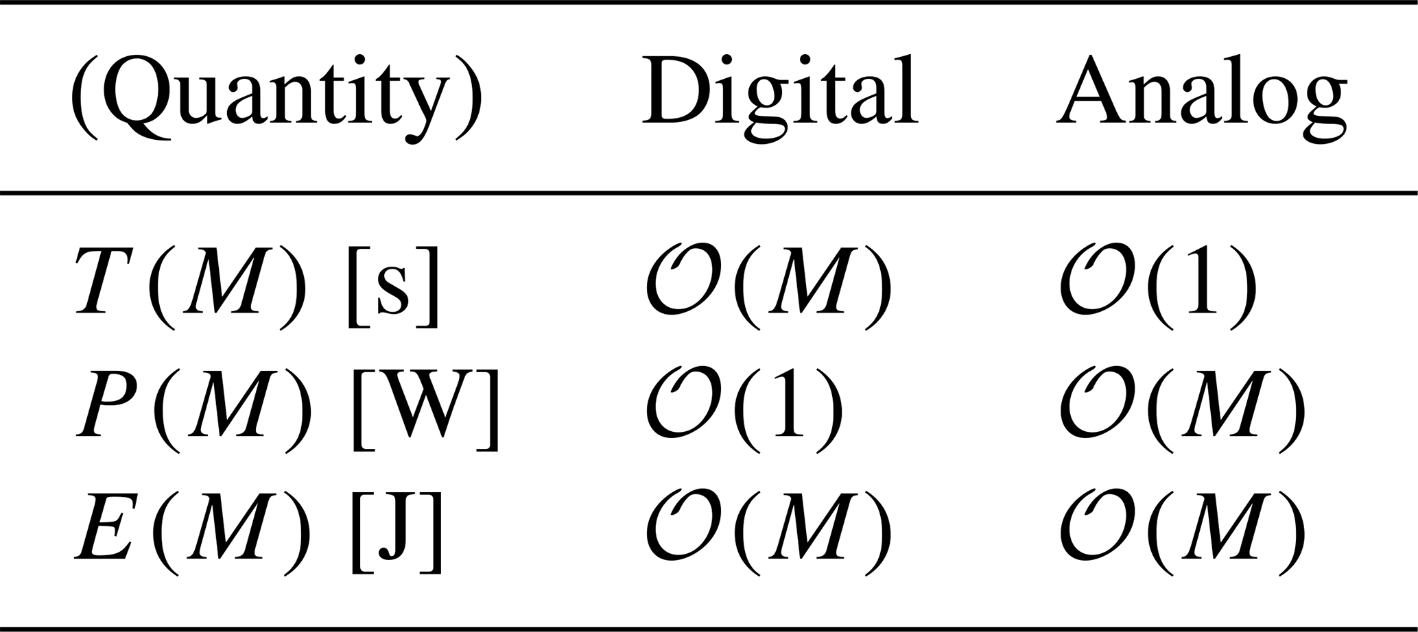
Table 1 A linear model for work: The computational cost C of evaluating f(u) in the ODE $\partial u/\partial t=f\left(u\right)$ is expected to grow as C∈𝒪(M). The effects on time-to-solution T, power P and energy E demands are shown.

When comparing digital and analog computer power consumption, the power consumption under consideration should include the total computer power including administrative parts (like network infrastructure, analog-to-digital converters or cooling) and power supplies. In this work, data of heterogenous sources are compared and definitions may vary.

2.3 Criticism and outlook

Given that the digital and analog technology (electric representation of information, transistor-based computation) is quite similar, the model prediction of a similarly growing energy demand is useful. Differences are of course hidden in the constants (prefactors) of the asymptotic notation 𝒪(M). Quantitative studies in the next sections examine this prefactor in 𝒪(M).

The linear model is already limited in the case of serial digital processors when the computation gets memory bound (instead of CPU-bound). Having to wait for data leads to a performance drop and might result in a worsened superlinear $T_{\mathrm{D}}^M$.

Parallel digital computing as well as serial analog computing has not yet been subject of the previous discussion. While the first one is a widespread standard technique, the second one refers to analog-digital hybrid computing which, inter alia, allows a small analog computer to be used repeatedly on a large problem, effectively rendering the analog part as an analog accelerator or co-processor for the digital part. Parallel digital computing suffers from a theoretical speedup limited due to the non-parallel parts of the algorithm (see also Gustafson, 1988), which has exponential impact on $T_{\mathrm{D}}^M$. This is where the intrinsically parallel analog computer exhibits its biggest advantages. Section 4 discusses this aspect of analog computing.

3 A performance survey on solving ordinary differential equations (ODEs)

In this section, quantitative measurements between contemporary analog and digital computers will be made. We use the Analog Paradigm Model-1 computer (Ulmann, 2019, 2020), a modern modular academic analog computer and an ordinary Intel© Whiskey Lake “ultra-low power mobile” processor (Core i7-8565U) as a representative of a typical desktop-grade processor. Within this experiment, we solve a simple¹ test equation ${\mathrm{d}}^{\mathrm{2}}y/\mathrm{d}{t}^{\mathrm{2}}=\mathit{\lambda }y$ (with real-valued y and $\mathit{\lambda }=\pm \mathrm{1}$) on both a digital and analog computer.

3.1 Time to solution

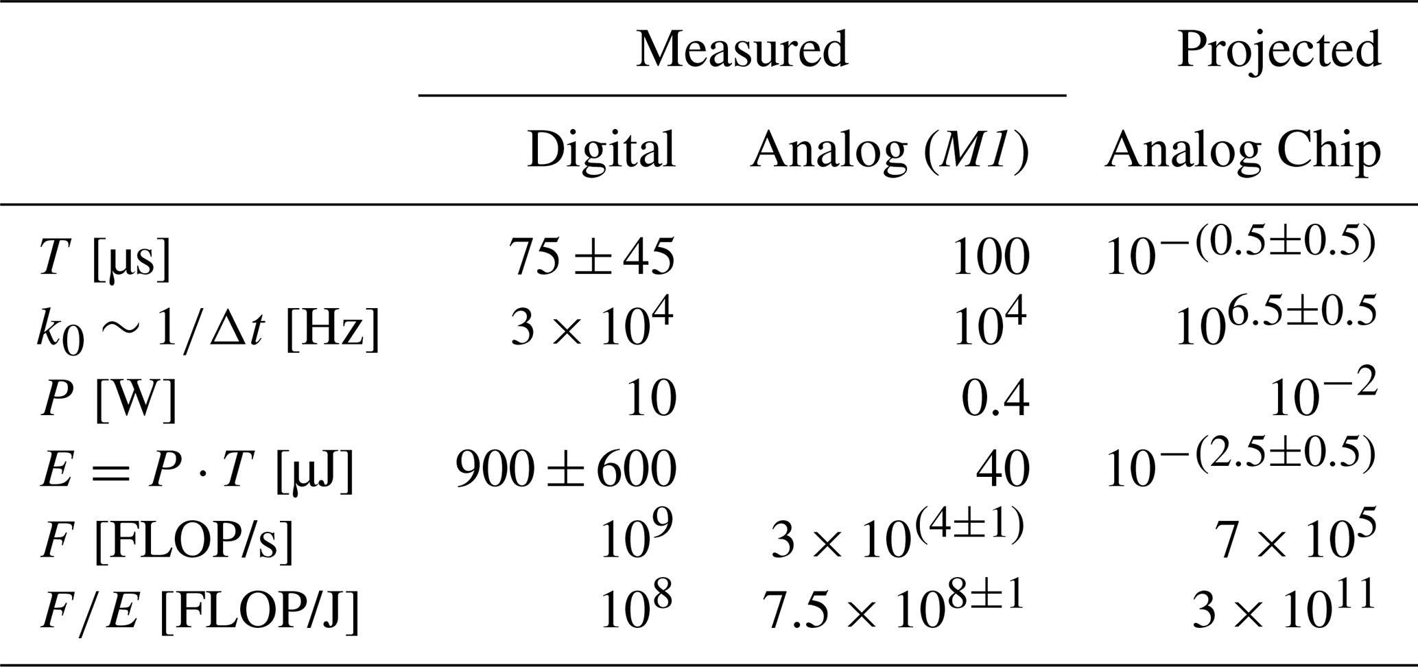
The digital computer solved the simple ordinary differential equation (ODE) with simple text-book level scalar benchmark codes written in C and Fortran and compiled with GCC. Explicit (forward) integrator methods are adopted (Euler/Runge-Kutta). The algorithm computed $N=\mathrm{2}\times {\mathrm{10}}^{\mathrm{3}}$ timesteps with timestep size $\mathrm{\Delta }t=\mathrm{5}\times {\mathrm{10}}^{-\mathrm{4}}$ each (see also Sect. 4 for a motivation for this time step size). Therefore, it is $t_{\mathrm{final}}=N\mathrm{\Delta }t=\mathrm{1}$. No output² was written during the benchmark to ensure the best performance. The time per element update (per integration step) was roughly (45±35) ns. For statistical reasons, the computation was repeated and averaged 10⁵ times. Depending on the order of the integration scheme, the overall wall clock time was determined as $T_{\mathrm{D}}=(\mathrm{75}\pm \mathrm{45})$ µs in order to achieve the simulation time t_final.

In contrast, the equation was implemented with integrating (and negating, if $\mathit{\lambda }=-\mathrm{1}$) operational amplifiers on the Analog Paradigm Model-1. The machine approached t_final=1 in a wall-clock time $T_A=\mathrm{1}\mathrm{s}/k_{\mathrm{0}}$ with $k_{\mathrm{0}}\in \mathit{\{}\mathrm{1},\mathrm{10},{\mathrm{10}}^{\mathrm{2}},{\mathrm{10}}^{\mathrm{3}},{\mathrm{10}}^{\mathrm{4}}\mathit{\}}$ the available integration speed factors on the machine (Ulmann, 2019). The Analog Paradigm Model-1 reached the solution of $y^{\prime \prime }=y$ at t_final=1 in a wall-clock time T_A=100 µs at best.

Note how $T_A/T_{\mathrm{D}}\approx \mathrm{1}$, i.e., in the case of the smallest possible reasonable ODE, the digital computer (2020s energy efficient desktop processor) is roughly as fast as the Analog Paradigm Model-1 (modern analog computer with an integration level comparable to the 1970s).

Looking forward, given the limited increase in clock frequency, with a faster processor one can probably expect an improvement of T_D down to the order of 1 µs. For an analog computer on a chip, one can expect an improvement of T_A down to the order of 1 µs–10 ns. This renders $T_A/T_{\mathrm{D}}\approx {\mathrm{10}}^{-(\mathrm{1}\pm \mathrm{1})}$ as a universal constant.

Summing up, with the given numbers above, as soon as the problem complexity grows, the analog computer outperforms the digital one, and this advantage increases linearly.

3.2 Energy and power consumption

The performance measure codes likwid (Hager et al., 2010; Röhl et al., 2017; Gruber et al., 2020) and perf (de Melo, 2010) were used in order to measure the overall floating-point operations (FLOP) and energy usage of the digital processor. For the Intel mobile processor, this provided a power consumption of P_D=10 W during computing. This number was derived directly from the CPU performance counters. The overall energy requirement was then $E_{\mathrm{D}}=P_{\mathrm{D}}{T}_{\mathrm{D}}=(\mathrm{0.9}\pm \mathrm{0.6})$ mJ. Note that this number only takes the processor energy demands into account, not any other auxiliary parts of the overall digital computer (such as memory, main board or power supply). For the overall power consumption, an increase of at least 50 % is expected.

The analog computer energy consumption is estimated as P_A≈400 mW. The number is based on measurements of actual Analog Paradigm Model-1 computing units, in particular 84 mW for a single summer and 162 mW for a single integrator. The overall energy requirement is then $E_A=P_A{T}_A=\mathrm{40}$µJ.

Note that $P_{\mathrm{D}}/P_A\approx \mathrm{25}$, while $E_{\mathrm{D}}/E_A\approx (\mathrm{2.25}\pm \mathrm{1.5})$. The conclusion is that the analog and digital computer require a similar amount of energy for the given computation, a remarkable result given the 40-year technology gap between the two architectures compared here.

For power consumption, it is hard to give a useful projection due to the accumulating administrative overhead in case of parallel digital computing, such as data transfers, non-uniform memory accesses (NUMA) and switching networking infrastructure. It can be assumed that this will change the ratio $E_{\mathrm{D}}/E_A$ further in favor of the analog computer for both larger digital and analog computers. Furthermore, higher integration levels lower E_A: the Analog Paradigm Model-1 analog computer is realized with an integration level comparable with 1970s digital computers. We can reasonably expect a drop of two to three orders of magnitude in power requirements with fully integrated analog computers.

3.3 Measuring computational power: FLOP per Joule

For the digital computer, the number of computed floating-point operations (FLOP³) can be measured. The overall single core nonvectorized performance was measured as $F\approx \mathrm{1}\mathrm{GFLOP}/\mathrm{s}$. A single computation until t_final required roughly F_D=3 kFLOP. The ratio $F_{\mathrm{D}}/P_{\mathrm{D}}=\mathrm{100}\mathrm{MFLOP}/\mathrm{J}$ is a measure of the number of computations per energy unit on this machine. This performance was one to two orders less than typical HPC numbers. This is because an energy-saving desktop CPU and not a high-end processor was benchmarked. Furthermore, this benchmark was by purpose single-threaded.

In this non-vectorized benchmark, the reduced resolution of the analog computer was ignored. In fact it is slightly lower than an IEEE 754 half precision floating-point, compared to the double precision floating-point numbers in the digital benchmark. One can then assign the analog computer a time-equivalent floating-point operation performance

$$\begin{array}{}\text{(5)}& F_A:=F_{\mathrm{D}}{\displaystyle \frac{T_A}{T_{\mathrm{D}}}}\approx {\mathrm{10}}^{(\mathrm{1}\pm \mathrm{1})}{F}_{\mathrm{D}}=\mathrm{3}\times {\mathrm{10}}^{(\mathrm{4}\pm \mathrm{1})}\mathrm{FLOP}.\end{array}$$

The analog computer FLOP-per-Joule ratio (note that $\mathrm{FLOP}/\mathrm{J}=\mathrm{FLOPs}/\mathrm{W}$) is

$$\begin{array}{}\text{(6)}& {\displaystyle \frac{F_A}{E_A}}={\displaystyle \frac{\mathrm{3}\times {\mathrm{10}}^{(\mathrm{4}\pm \mathrm{1})}\mathrm{FLOP}}{\mathrm{40}\mathrm{\mu }\mathrm{J}}}=\mathrm{7.5}\times {\mathrm{10}}^{\mathrm{8}\pm \mathrm{1}}\mathrm{FLOP}/\mathrm{J}.\end{array}$$

That is, the analog computer's “FLOP per Joule” is slightly larger than for the digital one. Furthermore, one can expect an increase of $F_A/E_A$ by 10–100 for an analog computer chip. See for instance Cowan (2005) and Cowan et al. (2005), who claim $\mathrm{20}\mathrm{GFlop}/\mathrm{s}$. We expect $\mathrm{300}\mathrm{GFlop}/\mathrm{s}$ to be more realistic, thought (Table 2).

Table 2 Small scaling summary: Measured benchmark (Intel© processor vs. Analog Paradigm Model-1) and expected/projected analog chip results.

Keep in mind that the FLOP/s or FLOP/J measures are (even in the case of comparing two digital computers) always problem/algorithm-specific (i.e., in this case a Runge Kutta solver of $y^{\prime \prime }=y$) and therefore controversial as a comparative figure.

4 PDEs and many degrees of freedom

This section presents forecasts about the solution of large scale differential equations. No benchmarks have been carried out, because a suitable integrated analog computer on chip does not yet exist. For the estimates, an analog computer on chip with an average energy consumption of about P_N=4 mW per computing element (i.e., per integration, multiplication, etc.) and maximum frequency ν=100 Mhz, which is refered to as the analog maximum frequency ν^A in the following, was assumed.was assumed.⁴ These numbers are several orders of magnitude better than the P_N=160 mW and ν=100 kHz of the Analog Paradigm Model-1 computer discussed in the previous section. For the digital part, different systems than before are considered.

In general, the bandwidth of an analog computer depends on the frequency response characteristics of the elements, such as summers and integrators. The actual achievable performance also depends on the technology. A number of examples shall be given to motivate our numbers: In 65 nm CMOS technology, bandwidths of over 2 GHz are achievable with integrators (Breems et al., 2016). At unity-gain frequencies of 800 MHz to 1.2 Ghz and power consumption of less than 2 mW, integrators with a unity-gain frequency of 400 Mhz are achievable (Wang et al., 2018).

4.1 Solving PDEs on digital and analog computers

Partial differential equations (PDEs) are among the most important and powerful mathematical frameworks for describing dynamical systems in science and engineering. PDE solutions are usually fields $\mathit{u}=\mathit{u}(\mathit{r},t)$, i.e., functions⁵ of spatial position r and time t. In the following, we concentrate on initial value boundary problems (IVBP). These problems are described by a set of PDEs valid within a spatial and temporal domain and complemented with field values imposed on the domain boundary. For a review of PDEs, their applications and solutions see for instance Brezis and Browder (1998). In this text, we use computational fluid dynamics (CFD) as a representative theory for discussing general PDE performance. In particular, classical hydrodynamics (Euler equation) in a flux-conservative formulation is described by hyperbolic conservation laws in the next sections. Such PDEs have a long tradition of being solved with highly accurate numerical schemes.

Many methods exist for the spatial discretization. While finite volume schemes are popular for their conservative properties, finite difference schemes are in general cheaper to implement. In this work, we stick to simple finite differences on a uniform grid with some uniform grid spacing Δr. The evolution vector field u(r,t) is sampled on G grid points per dimension and thus replaced by u_k(t) with $\mathrm{0}\le k<G$. It is worthwhile to mention that this approach works in classical orthogonal “dimension by dimension” fashion, and the number of total grid points is given by G^D. The computational domain is thus bound by $\mathrm{\Omega }=[{\mathit{r}}_{\mathrm{0}},{\mathit{r}}_G{]}^{\mathrm{D}}$. A spatial derivative ∂_if is then approximated by a central finite difference scheme, for instance ${\partial }_i{f}_k\approx (f_{k+\mathrm{1}}-f_{k-\mathrm{1}})/\left(\mathrm{2}\mathrm{\Delta }x\right)+\mathcal{O}\left(\mathrm{\Delta }{x}^{\mathrm{2}}\right)$ for a second order accurate central finite difference approximation of the derivative of some function f at grid point k.

Many algorithmic solvers implement numerical schemes which exploit the vertical method of lines (MoL) to rewrite the PDE into coupled ordinary differential equations (ODEs). Once applied, the ODE system can be written as ${\partial }_{\mathrm{t}}{u}^k=G^k(\mathit{u},\mathbf{\nabla }\mathit{u})$ with u^k denoting the time evolved (spatial) degrees of freedom and G^k functions containing spatial derivatives (∂_iu^j) and algebraic sources. A standard time stepping method determines a solution u(t₁) at later time t₁>t₀ by basically integrating $u^k\left(t_{\mathrm{1}}\right)={\int }_{t_{\mathrm{0}}}^{t_{\mathrm{1}}}{G}^k\left(\mathit{u}\right(t\left)\right)\mathrm{d}t+u^k\left(t_{\mathrm{0}}\right)$. Depending on the details of the scheme, G^k is evaluated (probably repeatedly or in a weak-form integral approach) during the time integration of the system. However, note that other integration techniques exist, such as the arbitrary high order ADER technique (Titarev and Toro, 2002, 2005). The particular spatial discretization method has a big impact on the computational cost of Gⁱ. Here, we focus on the (simplest) finite difference technique, where the number of neighbor communications per dimension grows linearly with the convergence order of the scheme.

4.2 Classical Hydrodynamics on analog computers

The broad class of fluid dynamics will be discussed as popular yet simple type of PDEs. It is well known for its efficient description of the flow of liquids and gases in motion and is applicable in many domains such as aerodynamics, in life sciences as well as fundamental sciences (Sod, 1985; Chu, 1979; Wang et al., 2019). In this text, the simplest formulation is investigated: the Newtonian hydrodynamics (also refered to as Euler equations) with an ideal gas equation of state. It is given by a nonlinear PDE describing the time evolution of a mass density ρ, it's velocity vⁱ, momentum pⁱ=ρvⁱ and energy $e=t+\mathit{\epsilon }$, with the kinetic contribution $t=\mathit{\rho }{\mathit{v}}^{\mathrm{2}}/\mathrm{2}$ and an “internal” energy ε, which can account for forces on smaller length scales than the averaged scale.

Flux conservative Newtonian hydrodynamics with an ideal gas equation of state are one of the most elementary and text-book level formulations of fluid dynamics (Toro, 1998; Harten, 1997; Hirsch, 1990). The PDE system can be written in a dimension agnostic way in D spatial dimensions (i.e., independent of the particular choice for D) as

$$\begin{array}{}\text{(7)}& {\displaystyle \frac{\partial \mathit{u}}{\partial t}}-\mathbf{\nabla }\cdot \mathit{f}=\mathit{S}\text{with}\mathbf{\nabla }\cdot \mathit{f}=\sum _i^{n_d}{\displaystyle \frac{\partial {\mathit{f}}^i}{\partial x^i}},\text{(8)}& {\displaystyle }\mathit{u}=\left(\begin{array}{l}\mathit{\rho }\\ p^j\\ e\end{array}\right),{\mathit{f}}^i={\mathit{f}}^i(\mathit{u},\mathit{v})=\left(\begin{array}{l}{p}^i\\ p^i{v}^j-p{\mathit{\delta }}^{ij}\\ v^i(e+p)\end{array}\right),\end{array}$$

with $i,j\in [\mathrm{1},D]$. Here, the pressure $p=\mathit{\rho }\mathit{\epsilon }(\mathrm{\Gamma }-\mathrm{1})$ defines the ideal gas equation of state, with adiabatic index Γ=2 and δ^ij is the Kronecker delta. A number of vectors are important in the following: The integrated state or evolved vector u in contrast to the primitive state vector or auxiliary quantities $\mathit{v}\left(u\right)=(p,v^i)$, which is a collection of so called locally reconstructed quantities. Furthermore, the right hand sides in Eq. (7) do not explicitly depend on the spatial derivative ∂ⁱρ, thus the conserved flux vector $\mathit{f}=\mathit{f}(\mathrm{\nabla }\mathit{q},\mathit{v})$ is only a function of the derivatives of the communicated quantities $\mathit{q}=(e,p^i)$ and the auxiliaries v. Furthermore, q and v are both functions of u only.

S=0 is a source term. Some hydrodynamical models can be coupled by purely choosing some nonzero S, such as the popular Navier Stokes equations which describe viscous fluids. Compressible Navier Stokes equations can be written with a source term $\mathit{S}=\mathbf{\nabla }\cdot {\mathit{F}}^v$, with

$$\begin{array}{}\text{(9)}& {\displaystyle }\text{diffusion fluxes}{\mathit{F}}^v=(\mathrm{0},{\mathit{\tau }}^{ij},{\sum }_k{\mathit{\tau }}^{ik}{v}^k-q^j{)}^T,\text{(10)}& {\displaystyle }\text{viscous stress}{\mathit{\tau }}^{ij}=\mathit{\mu }({\partial }^i{v}^j+{\partial }^j{v}^i-{\displaystyle \frac{\mathrm{2}}{\mathrm{3}}}({\partial }^k{v}^k\left){\mathit{\delta }}^{ij}\right),\text{(11)}& {\displaystyle }\text{and heat flux}{q}^i=-(c_p\mathit{\mu }/\mathrm{Pr}){\partial }^{i}T,\end{array}$$

with specific heats c_p, c_v, viscosity coefficient μ, Prandtl number Pr and temperature T determined by the perfect gas equation of state, i.e., $T=(e-{\mathit{v}}^{\mathrm{2}})/\left(\mathrm{2}{c}_v\right)$. The computational cost from Euler equation to Navier Stokes equation is roughly doubled. Furthermore, the partial derivatives on the velocities and temperatures also double the quantities which must be communicated with each neighbor in every dimension. We use Euler equations in the following section for the sake of simplicity.

4.3 Spatial discretization: Trading interconnections vs. computing elements

Schemes of (convergence) order F shall be investigated, which require the communication with F neighbour elements. For instance, a F=4th order accurate stencil has to communicate and/or compute four neighbouring elements ${\mathit{f}}_{k-\mathrm{2}},{\mathit{f}}_{k-\mathrm{1}},{\mathit{f}}_{k+\mathrm{1}},{\mathit{f}}_{k+\mathrm{2}}$. Typically, long-term evolutions are carried out with F=4 or F=6. In the following, for simplicity, second order stencil (F=2) is chosen. One identifies three different subcircuits

$$\begin{array}{}\text{(12)}& {\mathit{u}}_k({\mathit{f}}_{k+\mathrm{1}},{\mathit{f}}_{k-\mathrm{1}}):=\int \left({\mathit{f}}_{k+\mathrm{1}}-{\mathit{f}}_{k-\mathrm{1}}\right)\mathrm{d}\mathrm{t}/\left(\mathrm{2}\mathrm{\Delta }x\right),\end{array}$$

with ${\mathit{f}}_{k\pm \mathrm{1}}:={\mathit{f}}_k({\mathit{q}}_{k\pm \mathrm{1}},{\mathit{v}}_k)$ and v_k:=v_k(u_k) according to their previous respective definitions. Figure 1 shows this “building block” for a single grid point, an exemplar for up to D=2 dimensions with an F=2nd order finite difference stencil. The circuit identifies a number of intermediate expressions which are labeled as these equations:

$$\begin{array}{}\text{(13)}& \textcolor{red}{}\end{array}$$

Just like in Fig. 1, all expressions which are vanishing in a single spatial dimension are colored in red. Furthermore, note how the index i denotes the x-direction and k the y-direction, and that there are different fluxes f^j in the particular directions. Equation (13) is closed with the element-local auxiliary recovery

$$\begin{array}{}\text{(14)}& \textcolor{red}{}\end{array}$$

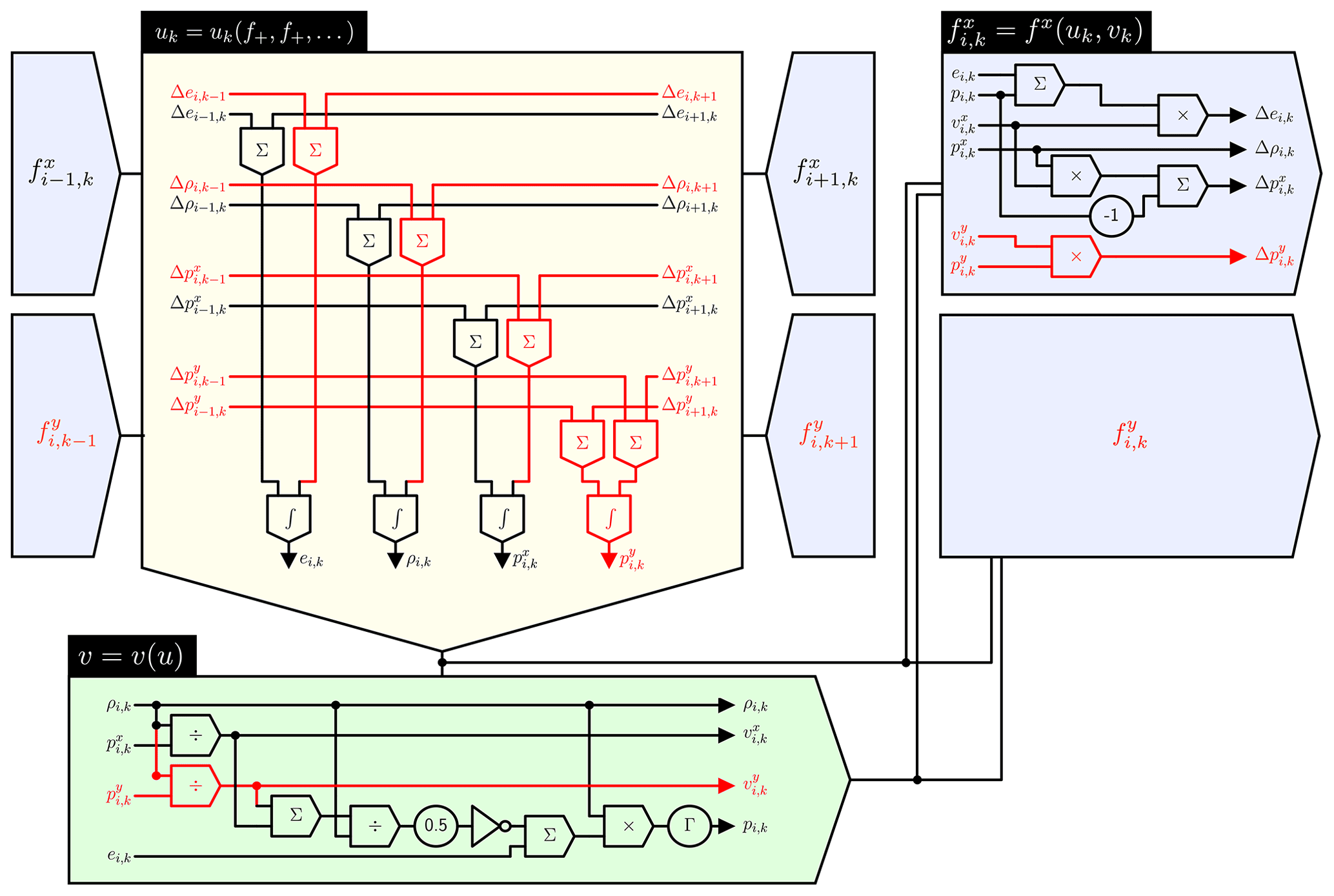
Figure 1 Overview circuit showing the blocks f, u and v. The three labeled blocks are distinguished by colour. Information flow is indicated with arrows. The overall circuit is given for lowest order (RK1) and in one spatial dimension. The red circuitry is the required addition for two spatial dimensions. All computing elements are drawn “abstractly” and could be directly implemented with (negating) operational amplifiers on a very large Analog Paradigm Model-1 analog computer.

Note that one can trade neighbor communication (i.e., number of wires between grid points) for local recomputation. For instance, it would be mathematically clean to communicate only the conservation quantities u and reconstruct v whenever needed. In order to avoid too many recomputations, some numerical codes also communicate parts of v. In an analog circuit, it is even possible to communicate parts of the finite differences, such as the Δv_i,k quantities in Eq. (13).

The number of analog computing elements required to solve the Euler equation on a single grid point is determined as $N_{\mathrm{single}}=\mathrm{5}D+\mathrm{5}F(D+\mathrm{2})+\mathrm{9}$, with D being the number of spatial dimensions and F the convergence order (i.e., basically the finite difference stencil size). Typical choices of interest are convergence orders of $F\in [\mathrm{2},\mathrm{6}]$ in $D\in [\mathrm{1},\mathrm{3}]$ spatial dimensions. Inserting the averaged $F=\mathrm{3}\pm \mathrm{1}$ and $D=\mathrm{2}\pm \mathrm{1}$ into N_single yields an averaged $N_{\mathrm{single}}\approx (\mathrm{84}\pm \mathrm{40})$ computing elements per spatial degree of freedom (grid point) required for implementing Euler equations.

Unfortunately, this circuit is too big to fit on the Analog Paradigm Model-1 computer resources available. Consequently the following discussion is based on a future implementation using a large number of interconnected analog chips. It is noteworthy that this level of integration is necessary to implement large scale analog computing applications. With P_N=4 mW per computing element, the average power per spatial degree of freedom (i.e., single grid point) is $P_{N\mathrm{D}}=(\mathrm{336}\pm \mathrm{160})$ mW.

4.4 Time to solution

Numerical PDE solvers are typically benchmarked using a wall-clock time per degree of freedom update measure T_DOF, where element update typically means a time integration timestep. In this measure, the overall wall clock time is normalized (divided) by the number of spatial degrees of freedom as well as the number of parallel processors involved.

The fastest digital integrators found in literature carry out a time per degree of freedom update $T_{\mathrm{DOF}}={\mathrm{10}}^{\mathrm{1}\pm \mathrm{1}}$ µs. Values smaller than 1 µs require already the use of sophisticated communication avoiding numerical schemes such as discontinuous Galerkin (DG) schemes.⁶ For instance, Dumbser et al. (2008) demonstrate the superiority of so called P_NP_M methods (polynomial of degree N for reconstruction and M for time integration, where the limit P₀P_M denotes a standard high-order finite volume scheme) by reporting T_DOF=0.8 µs for a P₂P₂ method when solving two-dimensional Euler equations. Diot et al. (2013) report an adaptive scheme which performs no faster than T_EU=30 µs when applied to three-dimensional Euler equations. The predictor-corrector arbitrary-order ADER scheme applied by Köppel (2018) and Fambri et al. (2018) to the general-relativistic magnetodynamic extension of hydrodynamics reported T_DOF=41 µs as the fastest speed obtained. The non-parallelizable evaluation of more complex hydrodynamic models is clearly reflected in the increasing times T_DOF.

Recalling the benchmark result of T_DOF∼45 ns from Sect. 3.1, the factor of 1000 is mainly caused by the inevitable communication required for obtaining neighbor values when solving f(y,∇y) in ${\partial }_{\mathrm{t}}y=f\left(y\right)$. Switched networks have an intrinsic communication latency and one cannot expect T_DOF to shrink significantly, even for newer generations of supercomputers. A key advantage of analog computing is that grid neighbor communication happens continuously in the same time as in the grid-local circuit. That is, no time is lost for communication.

One can do a comparison with the analog computer without knowing the simulation time step size Δt. The reasoning is based on the maximum frequency, i.e., the shortest wavelength which can be resolved with a (first order in time⁷) numerical scheme is $f_{\mathrm{sim}}:=\mathrm{1}/\left(\mathrm{10}\mathrm{\Delta }t\right)$, c.f., Fig. 2. The factor $\mathrm{10}=\mathrm{2}\cdot \mathrm{5}$ includes a factor of 2 due to the Nyquist-Shannon sampling theorem, while the factor of 5 is chosen to take into account that a numerical scheme can marginally reconstruct a wave at frequency $f=\mathrm{1}/\left(\mathrm{2}\mathrm{\Delta }t\right)$ by two points while it can be obtained perfectly by the analog computer (down to machine precision without any artifacts). The integration of signals beyond the maximum frequency results in a nonlinear response which heavily depends on the electrical details of the circuit (which are beyond the scope of the analog computer architecture discussed in this paper). One can demand that the numerical integrator time resolution is good enough to reconstruct a signal without prior knowledge on the wave form even at the maximum frequency.⁸ This drives the demand for 5 additional sampling points per half-wave, in order to make analog and digital outcome comparable (see also Fig. 2).

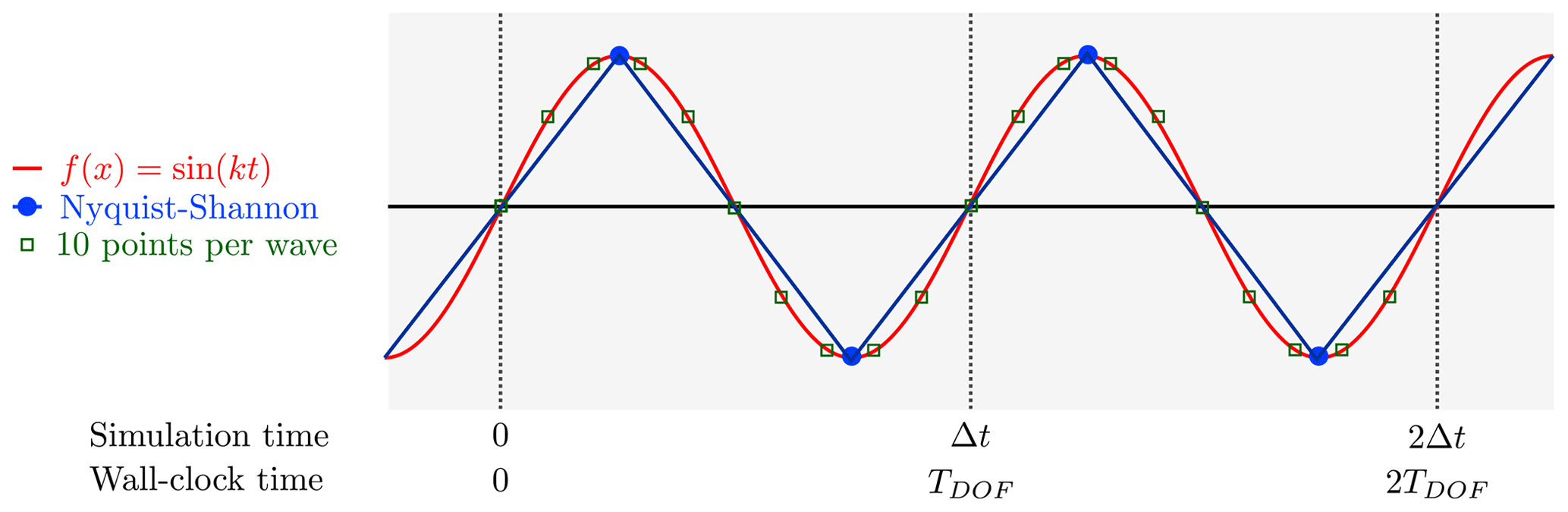
Figure 2 Analog signal sampling vs. numerical time integration: The time evolved sine with maximum frequency $k=\mathrm{2}\mathit{\pi }/\mathit{\lambda }$ has just the wavelength λ=Δt, with Δt being the timestep size of the explicit Euler scheme. The Nyquist-Shannon theorem allows to determine wave length and phase position with two sampling points per wave length. However, a first order reconstruction of numerical data shows a triangle (zigzag) function. In contrast, the full wave is clearly visible at analog integration. More sampling points close the gap between analog and numerical representation.

It is noted that this argument is relevant as long as one is interested in obtaining and preserving the correct time evolution (of a system described by the differential equation) with an analog or digital computer, respectively. In general, it is not valid to reduce the computational correctness within the solution domain of an initial value problem as this will invalidate any later solution.

By assigning the numerical PDE solver a maximum frequency identical to the highest frequency which can be evolved by the scheme in a given time, one introduces an effective digital computer maximum frequency

$$\begin{array}{}\text{(15)}& {\mathit{\nu }}^{\mathrm{D}}=\mathrm{1}/\left(\mathrm{10}{T}_{\mathrm{DOF}}\right)={\mathrm{10}}^{\mathrm{1}\pm \mathrm{1}}\mathrm{kHz}.\end{array}$$

Note how the mapping of simulation time (interval) Δt to wall-clock time (interval) T_DOF results in a mapping of simulation frequency f_sim to wall-clock (or real-time) frequency ν^D (Fig. 2).

The calculated ${\mathit{\nu }}^{\mathrm{D}}={\mathrm{10}}^{-\mathrm{2}\pm \mathrm{1}}$ MHz has to be contrasted with ν^A=100 MHz of the analog computer chip. One can conclude that analog computers can solve large scale high performance computing at least ${\mathit{\nu }}^A/{\mathit{\nu }}^{\mathrm{D}}={\mathrm{10}}^{\mathrm{3}\pm \mathrm{1}}$ times faster than the digital ones, when T_A and T_D are the analog and digital time to solution. Since $T\sim \mathrm{1}/\mathit{\nu }$, the resolution time reduces accordingly and $T_A/T_{\mathrm{D}}={\mathrm{10}}^{-\mathrm{3}\pm \mathrm{1}}$.

This is a remarkable result as it already assumes the fastest numerical integration schemes on a perfectly scaling parallel digital computer. In practical problems, these assumptions are hardly ever met: The impossibility of (ideal) parallelization is one of the major drawbacks of digital computing. Nevertheless, the above results show that even without these drawbacks, the analog computer is orders of magnitude faster. Notably, while it needs careful adjustment both the problem and the code for a high-performance computer to achieve acceptable parallel performance, when using an analog computer these advantages come effortless. The only way to reduce the speed or timing advantage is to choose a disadvantegeous or unsuitable number scaling.

In this study the low resolution of an analog computer (which is effectively IEEE 754 half precision floating-point) has been neglected. In fact, high order time integration schemes can invest computing time in order to achieve machine level accuracy which a typical error $\mathrm{\Delta }{f}_{\mathrm{digital}}\sim {\mathrm{10}}^{-\mathrm{10}}$ on some evolved function or field f and an error definition $\mathrm{\Delta }{f}_{\mathrm{simulation}}:=(f_{\mathrm{simulation}}-f_{\mathrm{exact}})/f_{\mathrm{exact}}$. An analog computer is limited by its intrinsic accuracy with a typical error $\mathrm{\Delta }{f}_{\mathrm{analog}}\sim {\mathrm{10}}^{-(\mathrm{4}\pm \mathrm{1})}$ (averaging over the Analog Paradigm Model-1 and future analog computers on chip).

4.5 Energy and power consumption

One expects the enormous speedup $T_A/T_{\mathrm{D}}$ of the analog computer to result in a much lower energy budget $E_{\mathrm{D}}=(T_{\mathrm{D}}/T_A)E_A={\mathrm{10}}^{\mathrm{3}\pm \mathrm{1}}{E}_A$ for a given problem. However, as the power requirement is proportional to the analog computer size, P_A=NP_ND, the problem size (number of grid points) which can be handled by the analog computer is limited by the overall power consumption. For instance, with a typical high performance computer power consumption of P_A=20 MW, one can simultaneously evolve a grid with $N=P_A/P_{N\mathrm{D}}={\mathrm{10}}^{\mathrm{11}\pm \mathrm{0.5}}$ points. This is in the same order of magnitude as the largest scale computational fluid dynamics simulations evolved on digital high performance computer clusters (c.f., Green 500 list, Subramaniam et al., 2013, 2020). Note that in such a setup, the solution is obtained on average 10^3±1 times faster with a purely analog computer and consequently also the energy demand is 10^3±1 times lower.

Just to depict an analog computer of this size: Given 1000 computing elements per chip, 1000 chips per rack unit, 40 units per rack still requires 2500 racks to build such a computer in a traditional design. This is one order of magnitude larger than the size of typical high performance centers. Clearly, at such a size the interconnections will also have a considerable power consumption, even if the monumental engineering challenges for such a large scale interconnections can be met. On a logical level, interconnections are mostly wires and switches (which require little power, compared to computing elements). This can change dramatically with level converters and an energy estimate is beyond the scope of this work.

4.6 Hybrid techniques for trading power vs. time

The analog computers envisaged so far have to grow with problem size (i.e., with grid size, but also with equation complexity). Modern chip technology could make it theoretically possible to build a computer with 10¹² analog computing elements, which is many orders of magnitude larger than any analog computer that has been built so far (about 10³ computing elements at maximum). The idea of combining an analog and a digital computer thus forming a hybrid computer featuring analog and digital computing elements is not new. With the digital memory and algorithmically controlled program flow, a small analog computer can be used repeatedly on a larger problem under control of the digital computer it is mated to. Many attempts at solving PDEs on hybrid computers utilized the analog computer for computing the element-local updated state with the digital computer looping over the spatial degrees of freedom. In such a scheme, the analog computer fulfils the role of an accelerator or co-processor. Such attempts are subject of various historical (such as Nomura and Deiters, 1968; Reihing, 1959; Vichnevetsky, 1968, 1971; Volynskii and Bukham, 1965; Bishop and Green, 1970; Karplus and Russell, 1971; Feilmeier, 1974) and contemporary studies (for instance Amant et al., 2014; Huang et al., 2017).

A simple back-of-the-envelope estimation with a modern hybrid computer tackling the N=10¹¹ problem is described below. The aim is to trade the sheer number of computing elements with their electrical power P, respectively, against solution time T. It is assumed that the analog-digital hybrid scheme works similarly to numerical parallelization: The simulation domain with N degrees of freedom is divided into Q parts which can be evolved independently to a certain degree (for instance in a predictor-corrector scheme). This allows to use a smaller analog computer which only needs to evolve $N/Q$ degrees of freedom at a time. While the power consumption of such a computer is reduced to $P_A\to P_A/Q$, the time to solution increases to T_A→QT_A. Of course, the overall required energy remains the same, $E_A=P_A{T}_A=(P_A/Q)\left(Q{T}_A\right)$.

In this simple model, energy consumption of the digital part in the hybrid computer as well as numerical details of the analog-digital hybrid computer scheme have been neglected. This includes the time-to-solution overhead introduced by the numerical scheme implemented by the digital computer (negligible for reasonably small Q) and the power demands of the ADC/DAC (analog-to-digital/digital-to-analog) converters (an overhead which scales with $(D+\mathrm{2})G^{\mathrm{D}}/Q$, i.e., the state vector size per grid element).

Given a fixed four orders of magnitude speed difference ${\mathit{\nu }}^{\mathrm{D}}/{\mathit{\nu }}^A={\mathrm{10}}^{\mathrm{4}}$ and a given physical problem with grid size N=10¹¹, one can build an analog-digital hybrid computer which requires less power and is reasonably small so that the overall computation is basically still done in the analog domain and digital effects will not dominate. For instance, with Q chosen just as big as $Q={\mathit{\nu }}^{\mathrm{D}}/{\mathit{\nu }}^A$, the analog computer would evolve only $N/Q={\mathrm{10}}^{\mathrm{7}}$ points in time, but run 10⁴ times “in repetition”. The required power reduces from cluster-grade to desktop-grade $P_A=(N/Q)P_{N\mathrm{D}}=\mathrm{3.3}$ kW. The runtime advantage is of course lost, $T_{\mathrm{D}}/T_A=\left(Q{\mathit{\nu }}^A\right)/{\mathit{\nu }}^{\mathrm{D}}=\mathrm{1}$.

Naturally, this scenario can also be applied to solve larger problems with a given grid size. For instance, given an analog computer with the size of N=10¹¹ grid points, one can solve a grid of size QN by succesively evolving Q parts of the computer with the same power P_A as for a grid of size N. Of course, the overall time to solution and energy will grow with Q. In any case, time and energy remain (3±1) orders of magnitude lower than for a purely digital computer solution.

5 Summary and outlook

In Sect. 2, we have shown the time and power needs of analog computers are orthogonal to those of digital computers. In Sect. 3, we performed an actual miniature benchmark of a commercially available Analog Paradigm Model-1 computer versus a mobile Intel© processor. The results are remarkable in several ways: The modern analog computer Analog Paradigm Model-1, uses integrated circuit technology which is comparable to the 1970s digital integration level. Nevertheless it achieves competitive results in computational power and energy consumption compared to a mature cutting-edge digital processor architecture which has been developed by one of the largest companies in the world. We also computed a problem-dependent effective FLOP/s value for the analog computer. For the key performance measure for energy-efficient computing, namely FLOP-per-Joule, the analog computer again obtains remarkable results.

Note that while FLOP/s is a popular measure in scientific computing, it is always application- and algorithm-specific. Other measures exist, such as transversed edges per second (TEPS) or synaptic updates per second (SUPS). Cockburn and Shu (2001) propose for instance to measure the efficiency of a PDE solving method by computing the inverse of the product of the (spatial-volume integrated) L¹-error times the computational cost in terms of time-to-solution or invested resources.

In Sect. 4, large scale applications were discussed on the example of fluid dynamics and by comparing high performance computing results with a prospected analog computer chip architecture. Large scale analog applications can become power-bound and thus require the adoption of analog-digital hybrid architectures. Nevertheless, with their 𝒪(1) runtime scaling, analog computers excel for time integrating large coupled systems where algorithmic approaches suffer from communication costs. We predict outstanding advantages in terms of time-to-solution when it comes to large scale analog computing. Given the advent of chip-level analog computing, a gigascale analog computer (a device with ∼10⁹ computing elements) could become a game changer in this decade. Of course, major obstacles have to be addressed to realize such a computer, such as the interconnection toplogy and realization in an (energy) efficient manner.

Furthermore, there are a number of different approaches in the field of partial differential equations which might be even better suited to analog computing. For instance, solving PDEs with artificial intelligence has become a fruitful research field in the last decade (see for instance Michoski et al., 2020; Schenck and Fox, 2018), and analog neural networks might be an interesting candidate to challenge digital approaches. Number representation on analog computers can be nontrivial when the dynamical range is large. This is frequently the case with fluid dynamics, where large density fluctiations are one reason why perturbative solutions fail and numerical simulations are carried out in the first place. One reason why indirect alternative approaches such as neural networks could be better suited than direct analog computing networks is that this problem is avoided. Furthermore, the demand for high accuracy in fluid dynamics can not easily fulfilled by low resolution analog computing. In the end, it is quite possible that a small-sized analog neural network might outperform a large-sized classical pseudo-linear time evolution in terms of time-to-solution and energy requirements. Most of these engineering challenges have not been discussed in this work and are subject to future studies.