 | 17 Dec 2021
Calculations of electromagnetic fields in longitudinal irregular TEM-cells
Hoang Duc Pham
Katja Tüting
Heyno Garbe
TEM-cells can be used as a standardized field generator for field probe calibration purposes or electromagnetic compatibility measurements. Because of its practical use as a measurement environment, the electromagnetic behavior over a broad range of frequencies is essential. However, without the understanding of wave reflection, mode-conversion, and attenuation, using such a measurement environment is impractical. In this contribution, we calculate the electromagnetic fields in a longitudinal irregular coaxial TEM-cell. Using a semi-analytical approach, we can determine these wave characteristics. The method is based on the projection of Maxwell's equations onto eigenfunctions. This work's primary objective is to examine the effect of irregular deformed boundaries on the electromagnetic field and the resonance frequencies.
- Article
(3905 KB) - Full-text XML
- BibTeX
- EndNote


An often-used field generator is the TEM-cell, a closed coaxial transmission line (Groh et al., 1999), as shown in Fig. 1. For reproducible electromagnetic compatibility (EMC) results, a suitable measurement environment and a particular field polarization are needed. It is desirable to measure the field strengths in the so-called far-field region. The fundamental mode in a TEM-cell is the TEM-mode; above a specific frequency fc (cutoff frequency), waveguide modes (TM and TE) start to propagate. So one primary downside is the upper-frequency limit. The TEM-cell consists of a uniform section tapered at each end to adapt to standard coaxial connectors (see Fig. 2). Usually, the TEM-cell is designed as a 50 Ω impedance-matched system to ensure minimum reflection of the operating TEM-mode. Due to the tapered sections, the waveguide modes will reflect at both ends. Thus, the TEM-cell forms a highly resonating structure. Another disadvantage compared to an open site or anechoic chamber is the limited test volume within the cell. Nevertheless, the electromagnetic (EM) field is well defined and sufficiently uniform to be useful in the calibration of EM field probes or EMC measurements. Higher frequency operation is achieved with a smaller TEM-cells cross-section 𝒮, but it also reduces the testing volume. The TEM-cell is used for creating a known EM field in which a field probe is calibrated for use as transfer standards or general-purpose field probes. Because such probes are usually small in their dimensions, and their calibration requires a very well-defined field, TEM-cells are a suitable field generator. A circular coaxial TEM-cell is of simple construction and basically an enlarged transmission line; it is also a portable measurement environment in its smaller versions (see Fig. 5).
However, practical TEM-cells are usually not uniform due to the geometry, e.g., surface roughness or tolerances in the manufacturing process. An efficient approach to calculate the EM fields in nonuniform waveguides is a semi-analytical method known as Generalized Telegraphist's Equations (GTEs). The GTEs and related methods of transverse cross-sections (also known as Coupled-mode theory and cross-section method) are widely used in the theory of waveguides with longitudinally varying boundaries (Shafii and Vernon, 1995; Vlasov and Antonsen, 2001; Maksimenko et al., 2019). By converting Maxwell's equations with appropriate boundary conditions (BCs), we obtain ordinary differential equations of the transmission line type (Schelkunoff, 1952). Expanding the EM fields into an orthogonal series of basis functions, an infinite system of differential equations is derived. Sporleder and Unger (1979), Huang and Hung-Chia (1984), and Katsenelenbaum et al. (1998) have published comprehensive monographs on this method. The previously mentioned works are mostly limited to waveguides with simply connected cross-sections.
Fliflet and Read (1981) originally derived the GTEs for coaxial waveguides. Koch (1999) has made the first attempt to thoroughly investigate closed TEM-Cells (Crawford- and GTEM-cells) using GTEs. The mode coupling mechanism in an ideal coaxial TEM-cell with circular cross-section has been investigated, and numerical results were shown in Pham and Garbe (2020). Because the GTEs can not directly calculate the resonance frequencies fr of the TEM-cells, an approximated method was presented in Pham et al. (2020).
In this contribution, the GTEs are used to investigate the effects of mechanical tolerances on the electromagnetic fields in coaxial TEM-cells. Therefore, the numerical results of the GTEs are verified by comparing them with a commercially available field simulator (CST Studio) and field measurements in a TEM-cell with similar geometric dimensions. The knowledge can be used in the design process of the TEM-cell to reduce mode-coupling and field uncertainties. In addition, the contribution of the field generator (TEM-cell) to the measurement uncertainty of electromagnetic fields can be determined, which is of great importance during field probe calibration.
First of all, we briefly introduce the theoretical formalism of the approach in Sect. 2. In Sect. 3, the irregular boundaries are modeled, and all relevant equations and parameters are derived. Following, Sects. 4 and 5, all numerical results are shown and discussed. The conclusion in Sect. 6 gives a summary of the most important insights of this contribution.

Figure 1Geometry of TEM-cell and schematic representation of measurement setup. The probe is located at .

As mentioned above, we concisely review the GTEs in this section, following prior published work (Pham and Garbe, 2020). To derive the GTEs for a two-port coaxial TEM-cell (see Fig. 1), we introduce a set of appropriate orthogonal coordinates . u and v are transverse coordinates, and for convenience, the z-axis coincides with the TEM-cells z-axis (see Fig. 2). We limit our analyses to an empty TEM-cell with the electric and magnetic constants (ε,μ). Next, we decompose the EM field vectors (E,H)
and the Nabla operator ∇
into transverse and longitudinal parts. and (Ez,Hz) are the transverse and longitudinal field amplitudes, and ∇⟂ is the Nabla operator for the transverse coordinates. We assume harmonic time dependence, and therefore the term ejωt (ω=2πf, carrier frequency) is omitted in all sequential equations. The transverse components of Maxwell's equations define E⟂ and H⟂ (Reiter, 1959)
Both transverse field components E⟂ and H⟂ will be expanded into a series of orthogonal vector functions (e,h). The transverse fields are represented at each axial location as a sum of the fundamental TEM-mode and the waveguides modes (TM- and TE-mode) with a transverse cross-section 𝒮 equal to the local cross-section of the reference TEM-waveguide. We have a solution in the following form
where (en,hn) are the eigenvector fields of the reference TEM-waveguide's electric and magnetic fields. The single subscript n in Eq. (4b) is considered a double subscript pq, where
To avoid the double summation expression, we will use the single subscript. For brevity, we will omit the index (TM, TE, and TEM) and distinguish between the different waveguide modes by enclosing the subscripts in parentheses (n) for TM-modes and in brackets [n] for TE-modes. The basis amplitudes (Vn(z),In(z)) are functions of the coordinate z. The eigenvector fields (e,h) in Eq. (4b) can be obtained by
where Π(u,v) is the scalar wavefunction (Marcuvitz, 1951). The different mode's scalar wavefunctions Π are determined by the following differential equations (Helmholtz and Laplace equation) and BCs
where denotes the Laplacian to the transverse coordinates. The term kn in Eqs. (7a) and (7b) describes the eigenvalue of the nth TM- or TE-mode.
The Poynting vector describes the power of the EM field. Concerning the orthogonality properties (9) and the series expansion (4b), we get
The surface integral is to be extended over the TEM-waveguide cross-section 𝒮 at z (see Fig. 2). We use the above expression (8) to simplify the entire representation and choose the eigenvector fields (en,hn) to satisfy the orthogonality condition
where δmn is the Kronecker delta function, and
is a normalization factor (Marcuvitz and Schwinger, 1951).
We use Maxwell's transverse components Eq. (3b), the modal expansion (4b), and the orthogonality condition (9) to derive the GTEs. Taking the projection on Maxwell's equations onto the eigenvector fields (e,h) results in an infinite set of ordinary differential equations (Vlasov and Antonsen, 2001)
in which γm is the propagation constant and Zm the wave impedance of the respective mode
The surface integrals on the right-hand side of Eq. (11b)
describe the effect of axial variations of the transverse cross-section 𝒮 (Reiter, 1959). The remaining line integrals in Eq. (11b) involve the tangential electric field at the boundary ∂𝒮. For the current case, we restrict our analysis to perfectly conducting TEM-cells (perfect electric conductor, PEC). Therefore, both terms become equal to zero using cylindrical coordinates and substituting the BCs (, PEC) into the integral kernel of Eq. (11b) (see Fig. 2)
The preceding Eq. (11b) apply to either TM-, TE-, or TEM-modes. A more detailed derivation of the GTEs can be seen in Marcuvitz and Schwinger (1951). In Pham and Garbe (2020), the mode coupling mechanism due to longitudinal variations of the geometry was reduced to TM0q- and TEM-mode coupling.
An analytical expression for the coupling coefficients C can be derived from the normalized eigenvector fields of a uniform coaxial TEM-waveguide. In our case, the coupling coefficients in Eq. (13) can be further simplified. We use the following boundary conditions for the scalar wavefunction Π (Solymar, 1959)
to reduce the surface integrals in Eq. (13) to line integrals over the cross-section's 𝒮 perimeter (Fliflet et al., 1980; Shafii and Vernon, 1995)
with
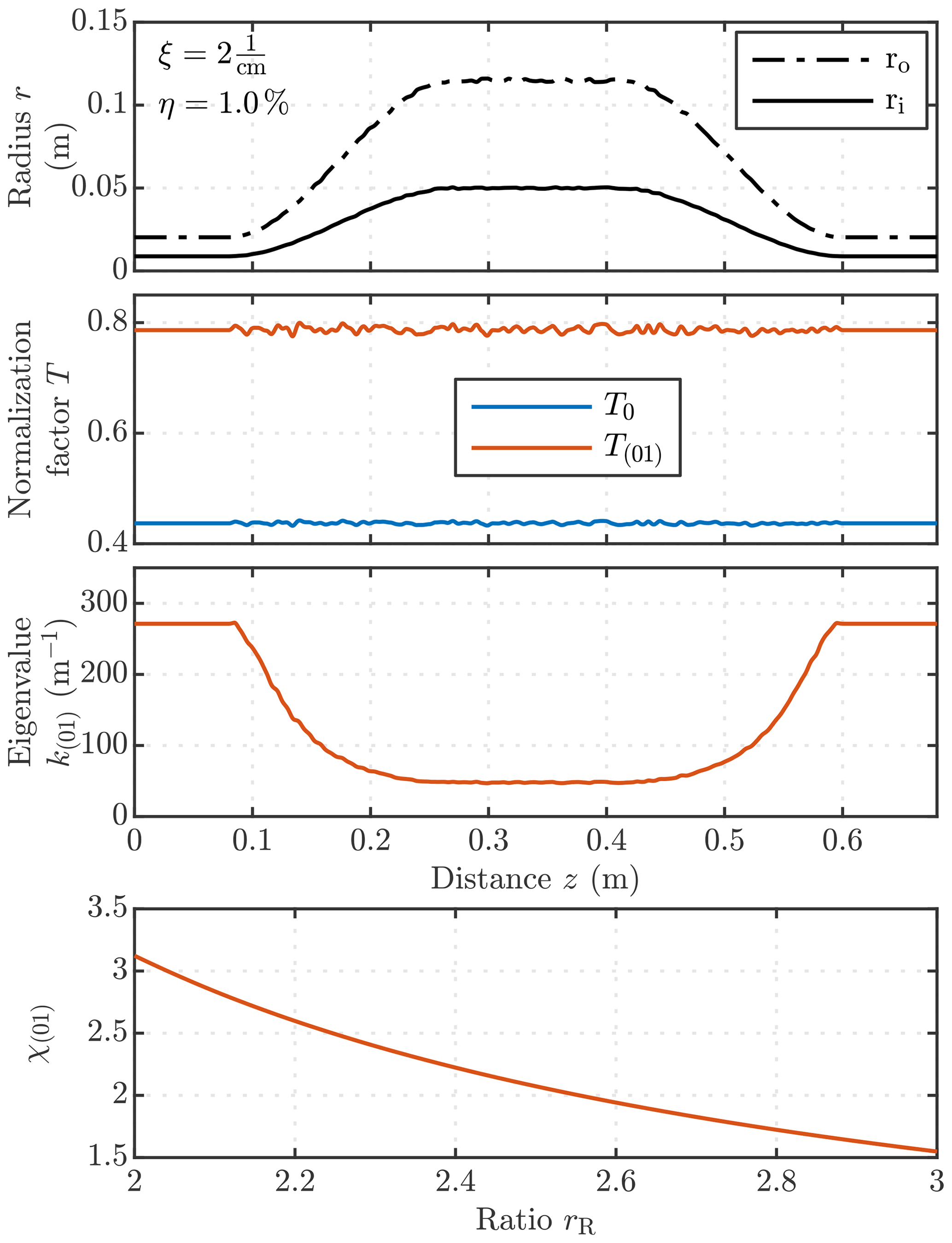
Figure 3One implementation of a longitudinal irregularly deformed TEM-cell and the resulting normalization factors (T0,T(01)) and the eigenvalue k(01). The terms ξ and η define the frequency and the amplitude of the perturbation along the TEM-cell. Below, the root χ(01) of the TM01-mode as a function of the ratio rR is shown.
According to Pham and Garbe (2020), TEM-cell's mode-coupling mechanism with longitudinal variations in the cross-section 𝒮 can be reduced to only interactions between TEM- and TM0q-modes. As long as the outer and inner radius ratio rR is constant along the z axis, no reflection of the operating TEM-mode occurs, and the coefficient in Eq. (16c) is zero. There is also no coupling to any higher-order TE-mode.
In Sect. 2, explicit formulas of the coupling coefficients were derived (see Eq. 16d). In the case of a longitudinal irregular TEM-cell, these coefficients do not change significantly. Due to the irregular inner and outer radius, the ratio
varies along the z axis. Hence the characteristic impedance
is not constant, which causes reflections of the operating TEM-mode. The coefficient C00 in Eq. (16c) becomes unequal zero. Another important fact is that the TM-modes eigenvalues
and both normalization factors
with
depend on the ratio rR(z). To calculate χ(pq) in Eq. (20), we need to compute the roots of the following equation (Marcuvitz, 1951)
In which Jp and Np denote to Bessel- and Neumann functions. As an illustrative example of a longitudinal irregular TEM-cell, the outer and inner radius (ro,i), the normalization factors (T0,T(01)), the eigenvalue k(01), and the root χ(01) are shown in Fig. 3. The radius ro,i is only a function of z
where Ro,i is the radius of the ideal TEM-cell, and the function δ describes the random deformation of the boundary.
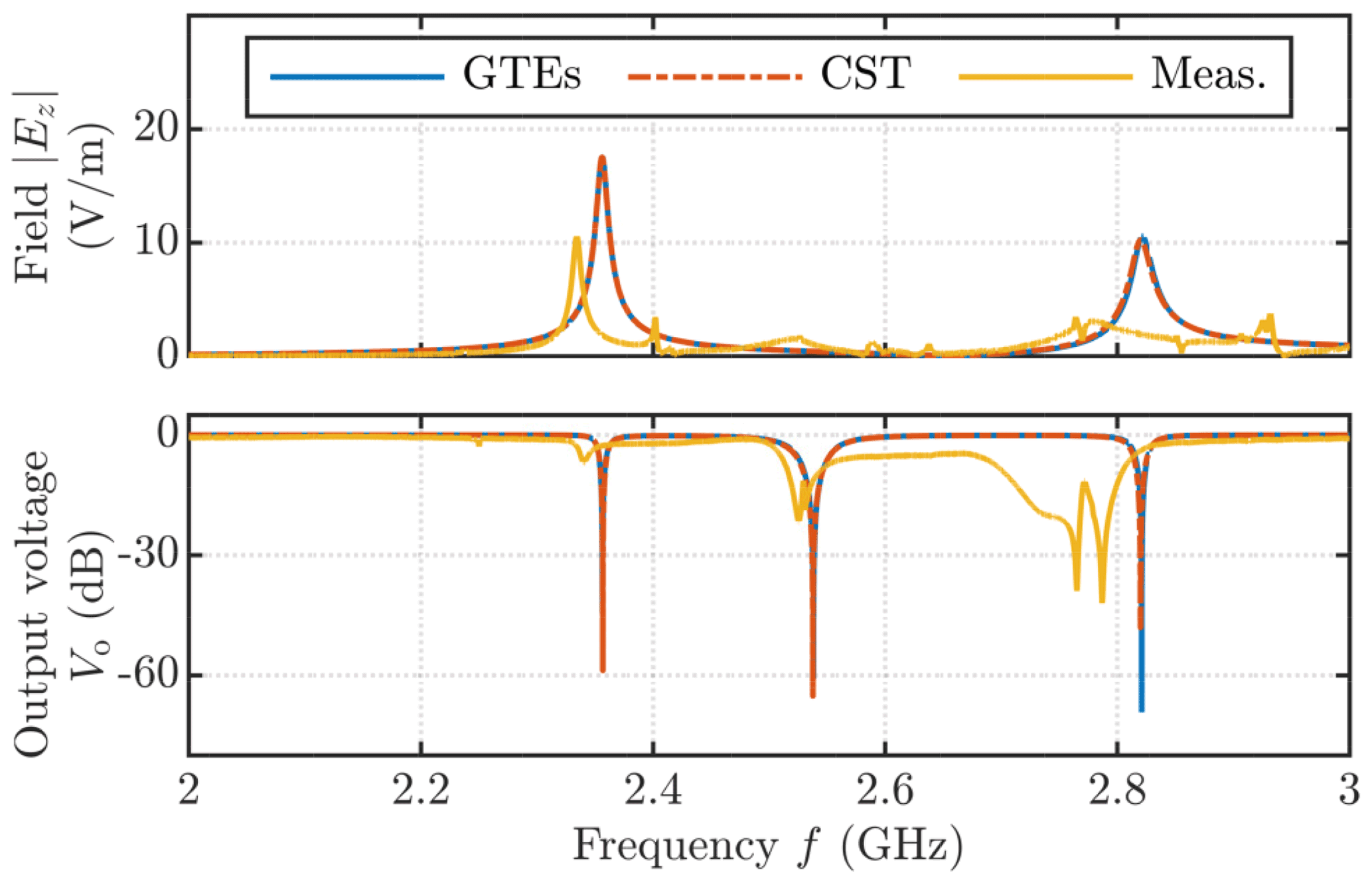
Figure 4Magnitude of the longitudinal field component and the output voltage Vo as a function of the frequency .
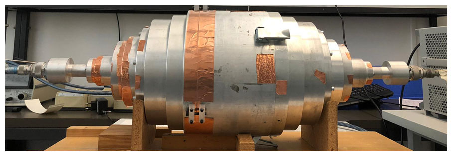
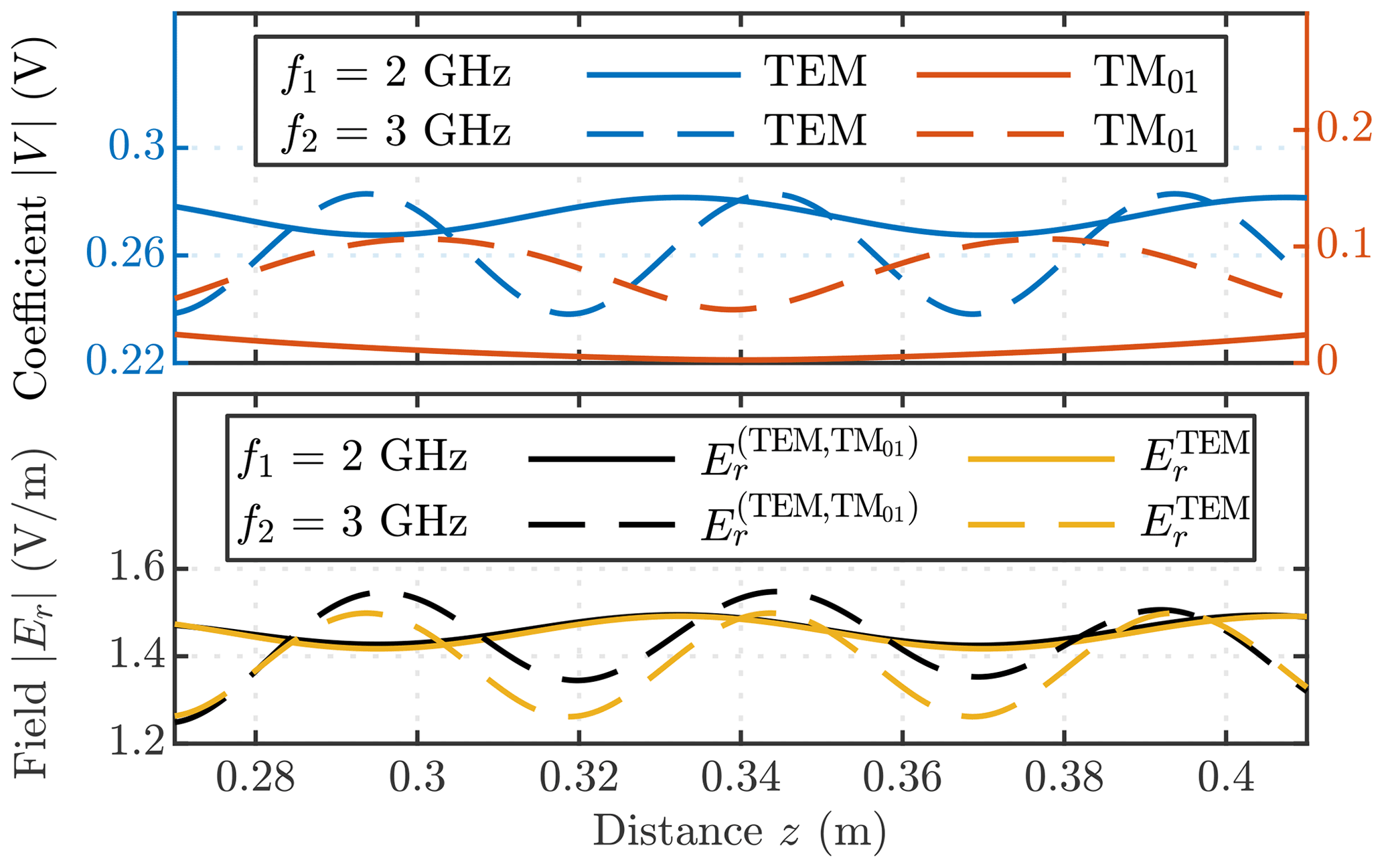
Figure 6Simulation results of the basis amplitudes (V0,V(01)) and the magnitude of the radial field component in between ro and ri at two frequencies (flow and fup).
To solve the GTEs of a two-port TEM-cell (see Fig. 1), we need additional BCs for the respective mode's basis amplitudes (V,I). The following BCs apply to the TEM-cells's left and the right port for the TEM-mode basis amplitude V0
For the basis amplitudes of the waveguide modes (TM and TE), the radiation conditions will be used at the TEM-cells in- and output (Fliflet and Read, 1981)
Wave impedances are used in the GTEs (Eq. 11b). Therefore, the characteristic impedance ZL needs to be substituted by the wave impedance Z0 in the above BCs (Eq. 25). The relation between both terms can be obtained by Eq. (19). According to the normalization of the basis amplitudes and eigenvectors (see Eqs. 9–8), Vq also needs to be substituted by
For coaxial TEM-waveguides with a concentric circular cross-section 𝒮, the transformation factor K becomes
Combining the two differential equations in Eq. (11b), we obtain the state space equation
The explicit form of the above matrices and vectors (V,I) can be found in Pham and Garbe (2020).
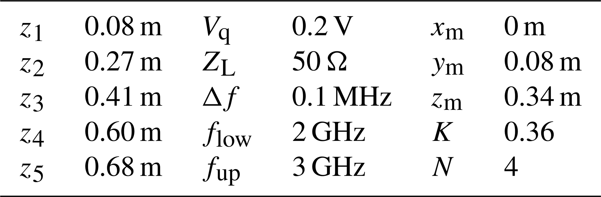
The infinite set of coupled differential equations (Eq. 29) is truncated and solved numerically by the finite difference method. In Pham and Garbe (2020), it has been shown that only four additional modes need to be considered in the frequency bandwidth for a coaxial TEM-cell with these geometric dimensions (see Fig. 1 and Table 2). Therefore, all our simulations were performed with N=4 modes. We have compared the longitudinal field component |Ez(rm)| and the output voltage Vo=|V0(z5)| of the GTEs with numerical results of another software tool and measurements on a coaxial TEM-cell with similar geometric dimensions. For the electric field measurements, we have used an optical field probe system (ENprobe EFs-105). A schematic setup of the measurement is given in Fig. 1. All results are displayed in Fig. 4.
The magnitude of the basis amplitudes V0,V(01) and V(02) for the upper and lower limit of our frequency bandwidth fb is displayed in Fig. 7. Using the GTEs, the resonance frequencies fr of the TEM-cell can be computed. We limited our simulations to a frequency step size of Δf=0.1 MHz, resulting in 10 001 frequency samples. The resonance frequencies fr can be obtained by analyzing the output voltage V0. Figure 8 shows the output voltage V0 as a function of the frequency f at the second port of an ideal and three implementation of an irregularly deformed TEM-cell. The transverse EM fields can be determined according to Eq. (4b). An analog expression for the longitudinal fields can be obtained by substituting Eq. (4b) into Maxwell's Equations (see Pham and Garbe, 2020). Figure 9 shows the magnitude of the radial and longitudinal electric field component as a function of the frequency along the z axis. The electric field magnitude is shown below the waterfall plots at the first resonance frequency along the radius r and the z axis.
Using the GTEs, the basis amplitudes (V,I) for different implementations of longitudinal irregularly deformed TEM-cells can be calculated, and a local probability density function (PDF) for the basis amplitudes can be obtained. As a representative example, 104 random implementations at fup were computed. The local PDF of the basis amplitude V0 is shown in Fig. 10a (only for the middle section of the TEM-cell). The mean value and the standard deviation of the basis amplitudes V0,V(01) and I(01) are given in Fig. 10b.

Figure 7Simulation results of the basis amplitudes V0,V(01) and V(02) at two different frequencies for an irregularly deformed TEM-cell.

Figure 8(a) Output voltage Vo at the second port (z=z5) for an ideal and three implementation of an longitudinal irregularly deformed TEM-cell. (b) As an illustrative example three implementation of an longitudinal irregularly deformed inner radius ri are shown. Because of the small deformation an additional zoom plot (blue box) is given for the middle section of ri.
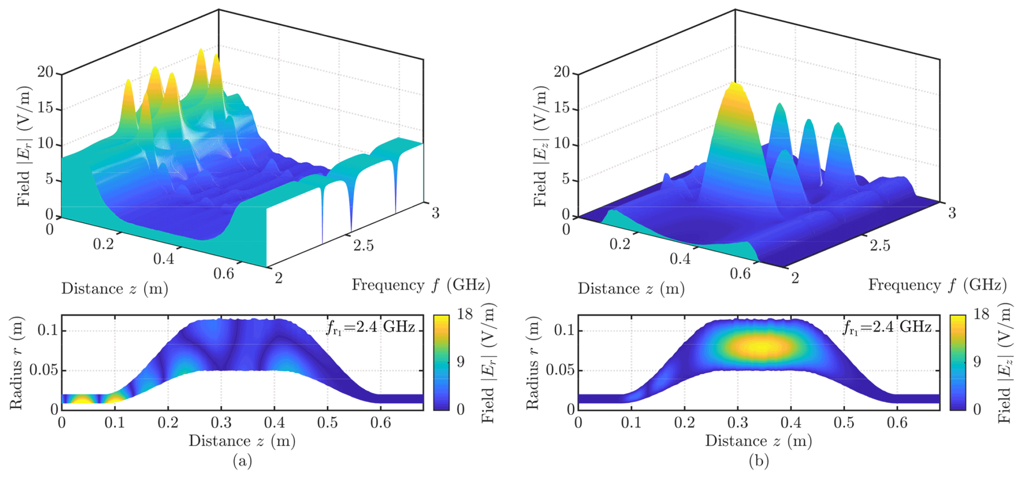
Figure 9(a) Magnitude of the radial field component in between ro and ri as a function of the frequency f. Below a cross-sectional view of |Er(r,z)| at the first resonance frequency . (b) Magnitude of the longitudinal field component in the center between ro and ri as a function of the frequency f. Below a cross-sectional view of |Ez(r,z)| at the first resonance frequency .
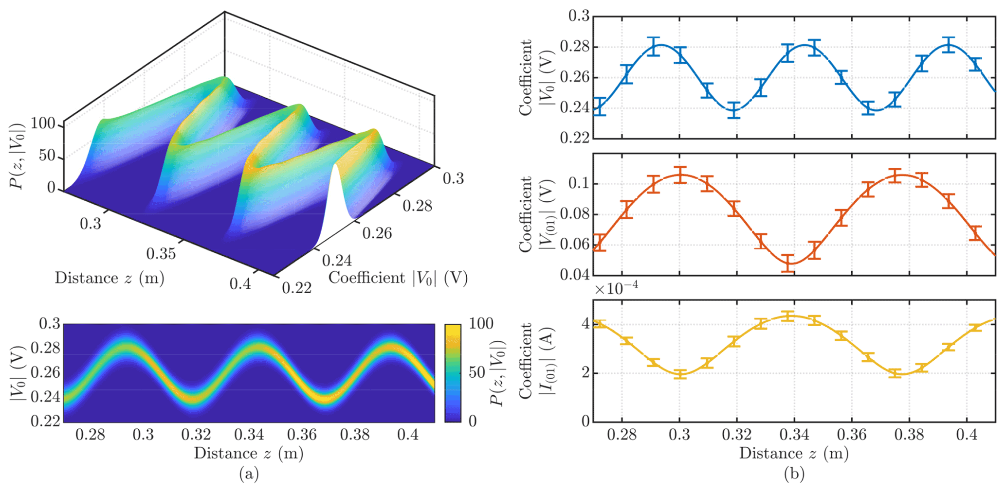
Figure 10(a) Local probability function of the basis coefficient V0 as a function of the distance z. (b) Mean value and standard deviation of the basis amplitudes V0,V(01) and I(01) as a function of the distance z.
Before examining the effect of longitudinal irregularly deformed boundaries on the EM fields and the resonance frequencies , we verified our numerical results of the GTEs for an ideal and regular TEM-cell.
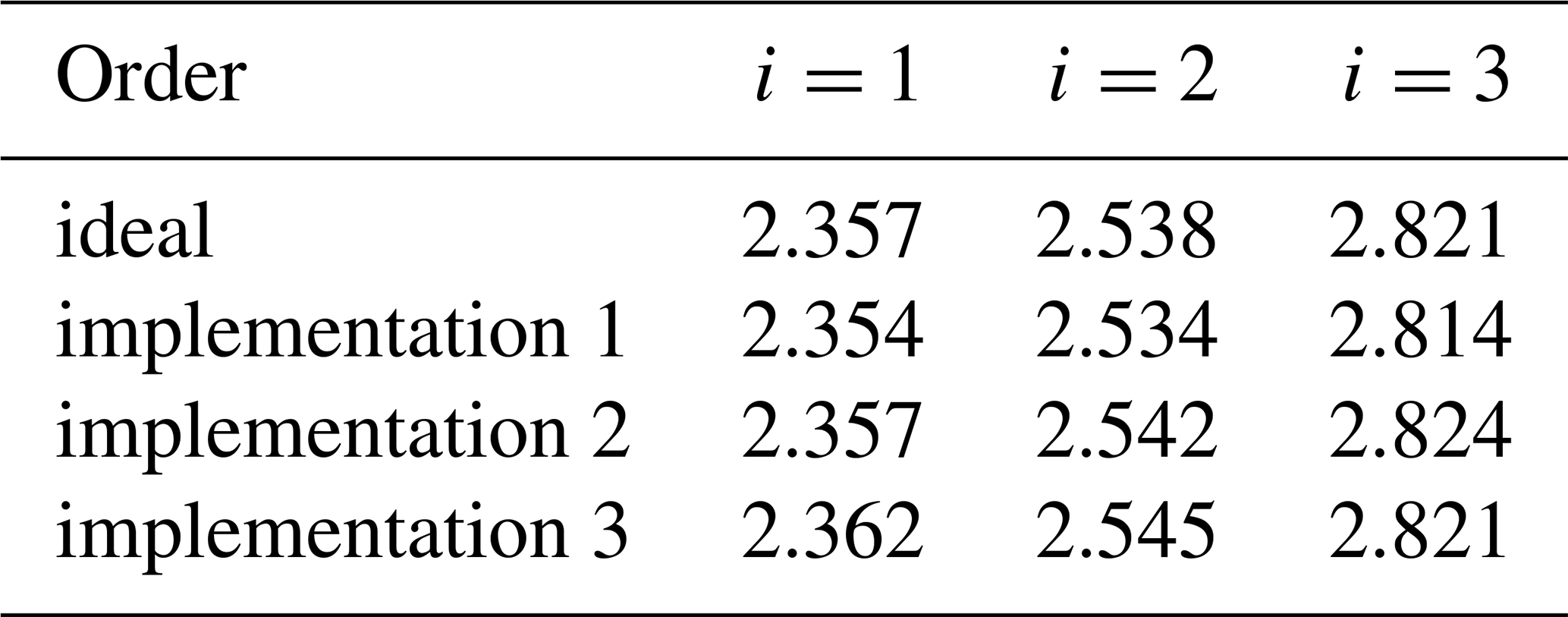
Table 2Resonance frequencies (GHz) of the TM01-mode in a coaxial TEM-cell with circular cross-section.
First, we compared the numerical results of the GTEs with simulations of commercially available software (CST Studio Suite 2019). The magnitude for the longitudinal electric field component |Ez(rm)| and the output voltage Vo=|V0(z5)| are in good agreement. Second, we conducted measurements on a TEM-cell with similar geometric dimensions (see Fig. 5). We can see some differences between the numerical results (GTEs and CST) and the measurements. Most likely due to various uncertainties during the measurement setup, e.g., position and alignment of the field probe, which have not been considered. The geometric uncertainties significantly impact the EM fields and resonance frequencies; for example, the tapering length and the coaxial connectors differ from our simulation model. Another critical factor is that we have limited our analyses to PEC, so all losses were neglected in the GTEs. Hence, the shift of the resonance frequencies is partially due to ohmic losses.
The obtained numerical results confirm strong mode-conversion from the operating TEM-mode to the TM01-mode, mostly in the tapered sections (see Fig. 7). Above the TM01-mode's cutoff frequency fc, the basis amplitude V(01) has a considerable magnitude and can not be neglected. In Fig. 6, the effect of the TM01-mode on the radial field component Er becomes apparent. A simple approximation of the radial field is possible since the basis amplitude V0 is dominant for most frequencies, except for the resonance frequencies (see Fig. 9). Due to the irregular boundaries, local coupling to higher-order TM0q-modes occurs throughout the TEM-cell. The deformed boundaries impact the course of the basis amplitudes and hence the field distribution (see Figs. 7 and 9). However, only the first propagating TM01-mode affects the middle section field because all basis amplitudes of the non-propagating modes are negligibly small. Additionally, we also have an impact on the resonance frequencies. A slight shift of all three resonance frequencies (up to 7 MHz) is notable (see Fig. 8 and Table 2).
In this contribution, the EM field and the resonance frequencies in a longitudinal irregular coaxial TEM-cell have been calculated using the GTEs. First of all, the coupling coefficients revealed the TEM-mode's effective mode-conversion in the tapered sections of the TEM-cell. Due to the irregular longitudinal boundaries along the TEM-cell, local excitation of the higher-order modes occurs. The magnitude of the coupling depends on the frequency. All calculations have been performed for a cylindrical TEM-cell with a circular cross-section, and numeric results were presented. The effect of irregularly deformed boundaries on the field and the resonance frequencies were shown. Comparable simulations and measurements on a coaxial TEM-cell with similar geometric dimensions have been performed to verify the results of the GTEs. Using the GTEs, we can calculate a local probability density function for the EM fields in the TEM-cell. Hence an uncertainty contribution due to the geometric tolerances of TEM-cell can be defined. The results can be used during the designing process of the TEM-cell to prevent higher-order mode coupling or estimate the uncertainty contribution of the field generator for a field probe calibration.
The simulation and measurement data are available on request.
HDP conceived the presented idea, developed the theoretical formalism, performed the analytic calculations, carried out the measurements, and wrote the manuscript. HDP and KT designed the model and the computational framework, planned and performed the numerical simulations, and analyzed it. HG was supervising the entire project and performed the final review. All authors discussed the results and contributed to the final manuscript.
The authors declare that they have no conflict of interest.
Publisher's note: Copernicus Publications remains neutral with regard to jurisdictional claims in published maps and institutional affiliations.
This article is part of the special issue “Kleinheubacher Berichte 2020”.
We thank Michael Koch, HS Hannover, for his assistance with the theoretical formalism. This work was supported by the cluster system, which is funded by the Leibniz Universität Hannover, the Lower Saxony Ministry of Science and Culture (MWK), and the German Research Association (DFG).
This research has been supported by the Deutsche Forschungsgemeinschaft (grant no. 438107418).
The publication of this article was funded by the open-access fund of Leibniz Universität Hannover.
This paper was edited by Madhu Chandra and reviewed by two anonymous referees.
Fliflet, A. W. and Read, M. E.: Use of weakly irregular waveguide theory to calculate eigenfrequencies, Q values, and RF field functions for gyrotron oscillators, Int. J. Electron., 51, 475–484, https://doi.org/10.1080/00207218108901350, 1981. a, b
Fliflet, A. W., Barnett, L. R., and Baird, J. M.: Mode Coupling And Power Transfer In A Coaxial Sector Waveguide With A Sector Angle Taper, IEEE T Microw. Theory, 28, 1482–1486, https://doi.org/10.1109/tmtt.1980.1130272, 1980. a
Groh, C., Kärst, J. P., Koch, M., and Garbe, H.: TEM waveguides for EMC measurements, IEEE T Electromagn. C, 41, 440–445, https://doi.org/10.1109/15.809846, 1999. a
Huang, H. and Hung-Chia, H.: Coupled Mode Theory: As Applied to Microwave and Optical Transmission, Taylor & Francis, Utrecht, the Netherlands, 1984. a
Katsenelenbaum, B. Z., del Rio, L. M., Pereyaslavets, M., Ayza, M. S., and Thumm, M.: Theory of Nonuniform Waveguides the cross-section method, The Institution of Electrical Engineers, London, United Kingdom, https://doi.org/10.1049/PBEW044E, 1998. a
Koch, M.: Analytische Feldberechnung in TEM-Zellen, Ph.D. thesis, Fachbereich Elektrotechnik und Informationstechnik, Leibniz Universität Hannover, Germany, 1999. a
Maksimenko, A. V., Shcherbinin, V. I., and Tkachenko, V. I.: Coupled-Mode Theory of an Irregular Waveguide with Impedance Walls, J. Infrared Millim. Te., 40, 620–636, https://doi.org/10.1007/s10762-019-00589-x, 2019. a
Marcuvitz, N.: Waveguide Handbook, IET Electromagnetic Waves Series 21, The Institution of Engineering and Technology, London, United Kingdom, https://doi.org/10.1049/PBEW021E, 1951. a, b
Marcuvitz, N. and Schwinger, J.: On the Representation of the Electric and Magnetic Fields Produced by Currents and Discontinuities in Wave Guides. I, J. Appl. Phys., 22, 806–819, https://doi.org/10.1063/1.1700052, 1951. a, b
Pham, H. D. and Garbe, H.: Mode Coupling in TEM-Cells due to Variations in the Geometry using Generalized Telegraphist's Equations, in: 2020 International Symposium on Electromagnetic Compatibility – EMC EUROPE, IEEE, https://doi.org/10.1109/emceurope48519.2020.9245825, 2020. a, b, c, d, e, f, g
Pham, H. D., Tüting, K., Garbe, H., and Koch, M.: A Method to Approximate the Resonance Frequencies of a Coaxial TEM-Cell, in: 2020 Asia-Pacific Microwave Conference – APMC Hong Kong, IEEE, 2020. a
Reiter, G.: Generalized telegraphist's equation for waveguides of varying cross-section, Proc. IEE – Part B: Electronic and Communication Engineering, 106, 54–61, https://doi.org/10.1049/pi-b-2.1959.0008, 1959. a, b
Schelkunoff, S. A.: Generalized Telegraphist's Equations for Waveguides, Bell Syst. Tech. J., 31, 784–801, https://doi.org/10.1002/j.1538-7305.1952.tb01406.x, 1952. a
Shafii, J. and Vernon, R. J.: Mode coupling in coaxial waveguides with varying-radius center and outer conductors, IEEE T. Microw. Theory, 43, 582–591, https://doi.org/10.1109/22.372104, 1995. a, b
Solymar, L.: Spurious Mode Generation in Nonuniform Waveguide, IEEE T. Microw. Theory, 7, 379–383, https://doi.org/10.1109/tmtt.1959.1124595, 1959. a
Sporleder, F. and Unger, H.-G.: Waveguide tapers, transitions, and couplers, P. Peregrinus on behalf of the Institution of Electrical Engineers, London, UK, 1979. a
Vlasov, A. N. and Antonsen, T. M.: Numerical solution of fields in lossy structures using MAGY, IEEE T. Electron. Dev., 48, 45–55, https://doi.org/10.1109/16.892166, 2001. a, b