Towards Steering Magnetic Nanoparticles in Drug Targeting Using a Linear Halbach Array

Magnetic nanoparticles offer numerous promising biomedical applications, e.g. magnetic drug targeting. Here, magnetic drug carriers inside the human body are directed towards tumorous tissue by an external magnetic field. However, the success of the treatment strongly depends on the amount of drug carriers, reaching the desired tumor region. This steering process is still an open research topic. In this paper, the previous study of a linear Halbach array is extended by an additional Halbach array with different magnetization angles between two adjacent magnets and investigated numerically using COMSOL Multiphysics. The Halbach arrays are arranged with permanent magnets and generate a relatively large region of a moderately homogeneous, high magnetic field while having a strong gradient. This results in a strong magnetic force, trapping many particles at the magnets. Afterwards, to avoid particle agglomeration, the Halbach array is flipped to its weak side. Therefore, the magnetic flux density, its gradient and the resulting magnetic force are computed for the different Halbach arrays with different constellations of magnetization directions. Since the calculation of the gradient can lead to high errors due to the used mesh in Comsol, the gradient was derived analytically by investigating two different fitting functions. Overall, the array with a 90^∘ shifted magnetization performs best, changing the magnetic sides of the array easily and deflecting more particles. Besides, the results revealed that the magnetic force dominates directly underneath the magnets compared to the other existing forces on the SPIONS. Summarized, the results depict that the magnetic force and, thus, the region where the particles are able to get washed out, can be adjusted using low-cost permanent magnets.

1 Introduction

In the last decades, the interest in steering superparamagnetic iron-oxide nanoparticles (SPIONs) to a desired location, particularly in the context of biomedical engineering, has grown rapidly (Nacev et al., 2012). SPIONs are supporting a great variety of diagnostic methods, e.g. as a contrast agent in magnetic resonance imaging (MRI; Vogel et al., 2020) or ultrasound (Fink et al., 2021), as well as therapeutic issues like in magnetic drug targeting (MDT; Alexiou et al., 2006) or hyperthermia (Mues et al., 2021). In MDT for example, the chemotherapeutic agents are bound to the SPIONs and injected into the cardiovascular system. Due to their magnetic properties, SPIONs can be pulled through the vessels into the tumorous tissue. This enables a local cancer treatment in a desired target volume, while at the same time side effects for the patient are reduced (Tietze et al., 2013). The resulting high efficiency of a MDT treatment was proven in an animal study by Tietze et al. (2013).

Nevertheless, the success of a MDT treatment strongly depends on the accumulation and therefore, on the ability to steer the SPIONs to the tumorous tissue. However, the required guiding is a complex problem, since it depends on various multiphysical parameters like the velocity profile of the blood flow, the gradient of the applied magnetic field as well as the properties of the nanoparticles themselves. The SPIONs should have a diameter of <200 nm to be able to penetrate into tissue and get not destroyed by the body's immune system (Zaloga et al., 2014). Since the magnetic force on the particles is proportional to the volume of one SPION, the forces are very weak due to their small size (Nacev et al., 2012). Furthermore, the particles need a coating with lipidic acids like lauric acid to be biocompatible and not agglomerating in blood (Zaloga et al., 2014), which decreases the possible size of the magnetic part inside the particles even more.

The main parameter for guiding a particle swarm through the cardiovascular system is the applied magnetic field. Here, the distance from the magnet between the SPIONs plays a crucial role, since the generated magnetic field decays approximately with $\mathrm{1}/R^{\mathrm{3}}$ and the magnetic force on one SPION depends on the magnitude and the gradient of the magnetic field. This leads to a trade-off between the magnetic field chosen too weak to attract enough SPIONs or one too strong, resulting in a scene, where most of the SPIONs get stuck inside the vessel underneath the magnet (Thalmayer et al., 2020). To overcome this problem, Park et al. (2020), Hoshiar et al. (2017), Kim et al. (2021) and many other authors proposed setups containing two or more electromagnets (EMs), which were placed at the opposite side of a vessel and switched on and off alternately. Nevertheless, EMs require a power supply in kW range, induce heat and have a weaker magnetic field (especially for the same volume) compared to rare earth permanent magnets (e.g. NdFeB; Bjørk et al., 2010, and Alnaimat et al., 2020). In contrast, permanent magnets yield the disadvantage that their magnetic field is constant and cannot be regulated or switched on and off. However, by using arrays of permanent magnets, the magnetic flux density can be adjusted by mechanical operations, like rotating the magnets (Bjørk et al., 2010). In the literature, Halbach configurations are well-established for this purpose, since their pattern produces the strongest magnetic flux density (Sakuma and Nakagawara, 2021). Baun and Blümler (2017) developed a coaxial arrangement of two Halbach arrays. It was further developed and is able to steer SPIONs precisely by rotating the arrays (Blümler, 2021).

In practice, however, it is not always possible to place the magnets surrounding the vessel. Thus, Thalmayer et al. (2021) introduced a configuration with a linear adjustable Halbach array (proposed by Hilton and McMurry, 2012), which is placed parallel to the vessel, for steering SPIONs through an Y-shaped bifurcation. The Halbach array contains a strong and a weak magnetic side, which can be switched by rotating the single magnets. This leads to an adjustable magnetic force. The basic idea is, having at first the strong magnetic side, and, thus, the strong magnetic force facing the vessel in order to pull as many particles as possible towards the magnets. Afterwards, the magnets are rotated so that the weak side points towards the vessel and, thus, the trapped particles are washed out by the fluid.

In this work, the results of the previous conference paper (Thalmayer et al., 2021) are extended and an additional Halbach configuration is investigated and compared to the primary adjustable Halbach array. For the calculation of the magnetic force, the magnetic flux density and its gradient are computed via fitting the simulation results, which is necessary due to high error peaks by deriving the magnetic flux density on a discrete mesh. This is done with two different functions. The corresponding fitting functions are additionally evaluated regarding the obtained errors and compared. All results were generated numerically using COMSOL Multiphysics^®.

2 Concepts and theory

To evaluate the precise steering of the SPIONs, two different arrangements of Halbach arrays are proposed in this section. Furthermore, the magnetic flux density of a Halbach array and the resulting forces acting on the particles in a MDT scenario, namely magnetic and hydrodynamic drag force, will be introduced.

2.1 Linear Halbach array configuration

In the literature, Halbach arrays are primarily utilized for electromotors (Zhang et al., 2011). However, in those setups, the Halbach array is usually coaxially arranged like in Shen and Zhu (2013). For separating particles, there is few research and also mostly in a coaxial arrangement (Blümler, 2021). However, Shiriny and Bayareh (2020), Stevens et al. (2021), Ijiri et al. (2013), and Kang et al. (2016) exemplary utilized a linear Halbach array for separating magnetic particles or cells. The results showed a stronger gradient and magnetic force compared to an array where the magnets were arranged with an alternating magnetization direction. However, their arrays were static, whereas in the proposed study, a linear Halbach array was utilized as an adjustable magnetic field source. Thus, the single magnets of the Halbach array are arranged to have a 90^∘ shifted magnetization compared to their direct neighbors. This leads to a one-sided magnetic field (see Fig. 1). By rotating the single magnets by $\mathit{\pi }/\mathrm{2}$ as depicted in Fig. 1, the strong and the weak side of the array can be changed. For the proposed configuration, Hilton and McMurry (2012) evaluated the torque $\mathit{N}=\mathit{m}\times \mathit{B}$ (Jackson, 1998) for the proposed configuration. They figured out that for a practical realization a mechanical stabilization is mandatory.

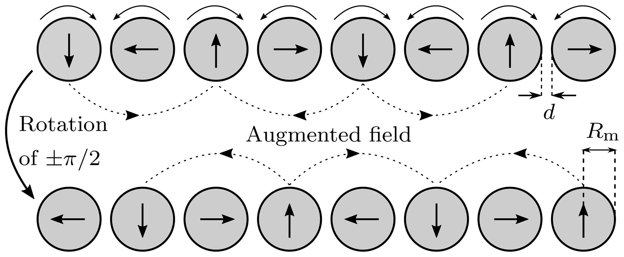
Figure 1 Magnetization pattern and field distribution of the adjustable Halbach array. The magnetic field can be shifted from below to above the magnets by changing φ from 0 to $\mathit{\pi }/\mathrm{2}$ (Reprinted with permission from Thalmayer et al., 2021; © IEEE).

2.2 Extended Halbach array

In extension to our previous published work (Thalmayer et al., 2021) of analyzing the adjustable Halbach array, an extended Halbach array is investigated for its performance on particle deflection. The magnets of this extended array have a 45^∘ shifted magnetization compared to their direct neighbors according to the setup displayed in Fig. 2. In the literature, Halbach arrays are used with several magnetization angles between two adjacent magnets (Zhang et al., 2011, or Shen and Zhu, 2013), however, as aforementioned the arrays are usually coaxial and not linear arranged. For the use case of particle deflection, to the best of the authors' knowledge currently only linear Halbach arrays with a magnetization shift of 90^∘ between each other were investigated. Therefore, the performance on the SPION deflection for an array with a 45^∘ shifted magnetization, is investigated.

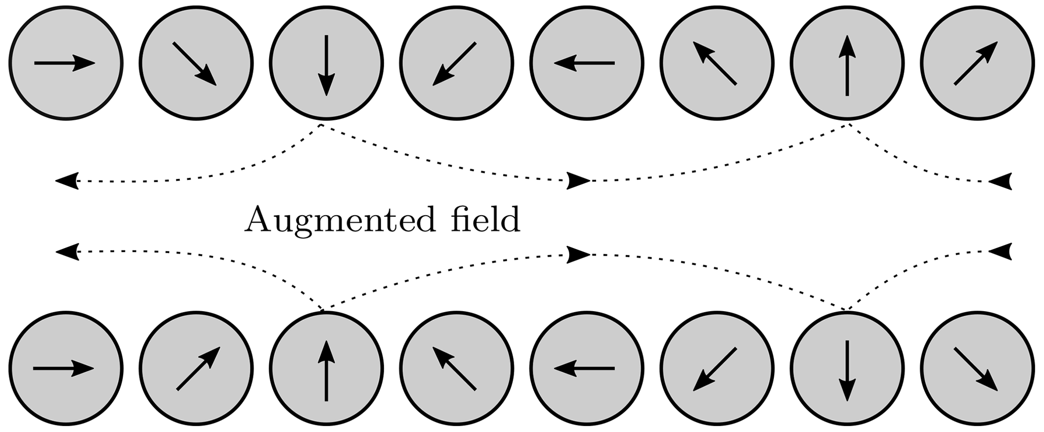
Figure 2 Magnetization pattern and field distribution of the extended Halbach array. Here, the two sides cannot be changed by a simultaneous rotation of all single magnets.

In the proposed extended array, the magnetic field of the extended Halbach array is augmented and attenuated on one side, respectively, like in the normal Halbach array in Fig. 1. However, in case of the extended Halbach array the strong and the weak side cannot be changed by a simultaneous rotation of all single magnets. Therefore, the mechanical rotation of the strong and the weak magnetic side is significantly more challenging.

2.3 Magnetic flux density of a Halbach array

Most approaches in the literature use numerical methods or programs such as COMSOL Multiphysics^® (Bjørk and Insinga, 2018; Ijiri et al., 2013) for determining the magnetic flux density B of a Halbach array. However, there are also analytic solutions (Peng and Zhou, 2013; Shen and Zhu, 2013; Zhang et al., 2020; Sim and Ro, 2020). For particle deflection the gradient of B is needed additionally. Calculating the gradient numerically often leads to high errors due to the meshwise computation of B, which is computed with Comsol in this work. Therefore, B is fitted with two variable functions for further investigations and, thus, the gradient can be derived analytically. The first function is adapted in accordance to the analytic solution of Sim and Ro (2020)

$$\begin{array}{}\text{(1)}& B={\displaystyle \frac{c_{\mathrm{1}}y+c_{\mathrm{2}}}{\left(c_{\mathrm{3}}{y}^{\mathrm{2}}+c_{\mathrm{4}}\right)\cdot \sqrt{c_{\mathrm{5}}{y}^{\mathrm{2}}+c_{\mathrm{6}}}}},\end{array}$$

where c_i with $i\in \left\{\mathrm{1},\mathrm{2},\mathrm{\dots },\mathrm{6}\right\}$ are arbitrary constants. Here, B is assumed to only have a component in the y-direction. The second fitting function is based on an exponential ansatz

$$\begin{array}{}\text{(2)}& B=k_{\mathrm{1}}{e}^{-k_{\mathrm{2}}y},\end{array}$$

which was already used in Thalmayer et al. (2021). Here, k₁ and k₂ correspond to arbitrary constants. The constants c_i and k_i are fitted for both, the Halbach and the extended Halbach array for the strong and the weak magnetic side. The fitting is done based on the simulation results from Comsol, by using a least square (LS) algorithm for every x.

2.4 Magnetic force

The resulting magnetic force F_mag on one SPION at a position r is defined by (Jackson, 1998)

$$\begin{array}{}\text{(3)}& {\mathit{F}}_{\mathrm{mag}}\left(\mathit{r}\right)=\mathbf{\nabla }\left(\mathit{m}\left(\mathit{r}\right)\cdot \mathit{B}\left(\mathit{r}\right)\right).\end{array}$$

Thereby, B [T] is the magnetic flux density at the location of the SPIONs with a magnetic moment m [A m²]. The magnetic moment m is given by the integral of the magnetization M over the particle's volume V (Jackson, 1998). Usually, the magnetization $M=M_{\mathrm{sat}}\cdot \mathcal{L}\left(\mathit{\xi }\right)$ is assigned to be homogeneous within a SPION and increases by a monotonic Langevin-function ℒ(ξ) (Baun and Blümler, 2017). ξ is directly proportional to B, whereas M_sat corresponds to the saturation magnetization. Since one SPION is only composed of a single magnetic domain, it shows no hysteretic behavior (Cullity and Graham, 2008). Alternatively to the magnetization M, the SPIONs can be characterized by their magnetic susceptibility χ (Baun and Blümler, 2017).

From Eq. 3 and the assumption of a homogeneous magnetization, it follows that the magnitude of the magnetic force $\left|{\mathit{F}}_{\mathrm{mag}}\right|$ depends on the volume V, the magnetization M and the gradient of the magnetic flux density G=∇B:

$$\begin{array}{}\text{(4)}& \left|{\mathit{F}}_{\mathrm{mag}}\right|=mG=VMG.\end{array}$$

The magnitude of $\left|{\mathit{F}}_{\mathrm{mag}}\right|$ for the application of MDT is usually in the range between 10⁻¹¹ to 10⁻²⁵ N (Nacev et al., 2012).

2.5 Hydrodynamic drag force

The (hydrodynamic) drag force on one spherical SPION is

$$\begin{array}{}\text{(5)}& {\mathit{F}}_{\mathrm{drag}}=\mathrm{6}\mathit{\pi }\mathit{\eta }{R}_{\mathrm{h}}\mathit{u}\end{array}$$

according to Baun and Blümler (2017), where η is the fluid's dynamic viscosity [Pa s]. R_h and u correspond to the hydrodynamic radius and the resulting velocity of one SPION, respectively. Since a low flow regime is assumed, other forces (like buoyant or lift force) on the SPIONs can be neglected (Thalmayer et al., 2020). The velocity profile u(y) is assumed to be laminar. Thus, the profile is parabolic and can be expressed by

$$\begin{array}{}\text{(6)}& u\left(y\right)=u_{\max }\left[\mathrm{1}-{\left({\displaystyle \frac{y}{R_v}}\right)}^{\mathrm{2}}\right],\end{array}$$

where u_max=2 u_mean. For blood, u_max varies between 0.5 mm s⁻¹ to 40 cm s⁻¹ (Nacev et al., 2012).

For a predominant movement of the SPIONs towards the magnets, the magnitude of the magnetic force F_mag has to be greater than the magnitude of F_drag:

$$\begin{array}{}\text{(7)}& \left|{\mathit{F}}_{\mathrm{mag}}\right|\stackrel{!}{\ge }\left|{\mathit{F}}_{\mathrm{drag}}\right|\iff VMG\stackrel{!}{\ge }\mathrm{6}\mathit{\pi }\mathit{\eta }{R}_{\mathrm{h}}u.\end{array}$$

In our proposed setup (see Fig. 3), F_mag and F_drag can be assumed to be perpendicular, as the changes of the magnetic flux density in the x-direction can be neglected. In consequence, G becomes

$$\begin{array}{}\text{(8)}& G={\displaystyle \frac{\mathrm{9}\mathit{\eta }u}{\mathrm{2}{R}_{\mathrm{p}}^{\mathrm{2}}M}}\end{array}$$

for an equilibrium of F_mag and F_drag. For sake of simplicity, the hydrodynamic radius R_h of one SPION is assumed to be equal to the magnetic particle radius R_p.

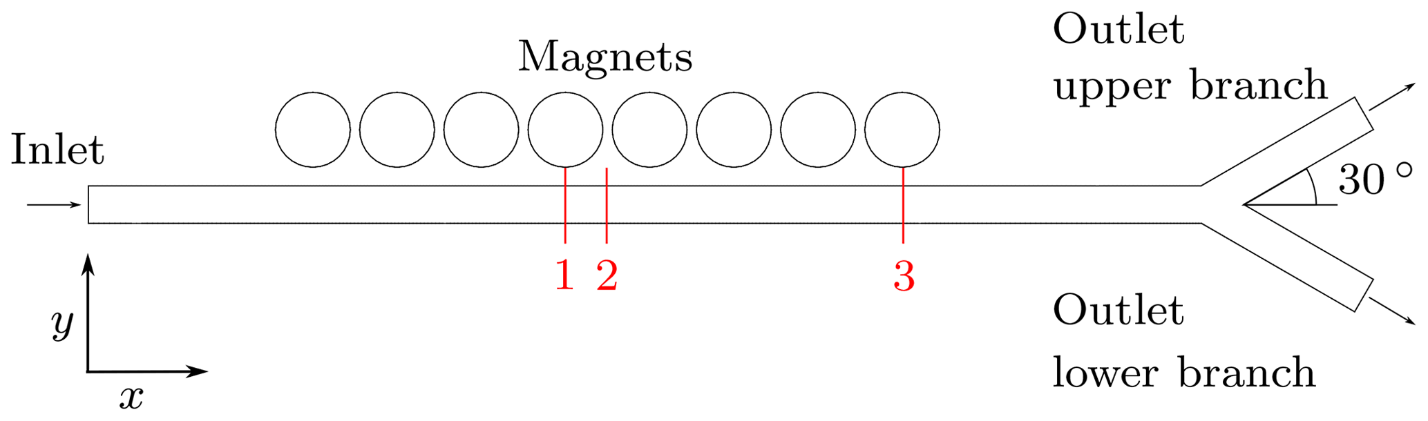
Figure 3 Proposed geometry model used in the 2D Comsol simulations. The magnetic field is analyzed at three positions, marked as red numbers. Whereas the measuring positions “1” and “3” are located underneath the fourth and the last magnet, respectively, “2” is located symmetrical in the center of the array at the gap between two adjacent magnets.

2.6 Simulation model

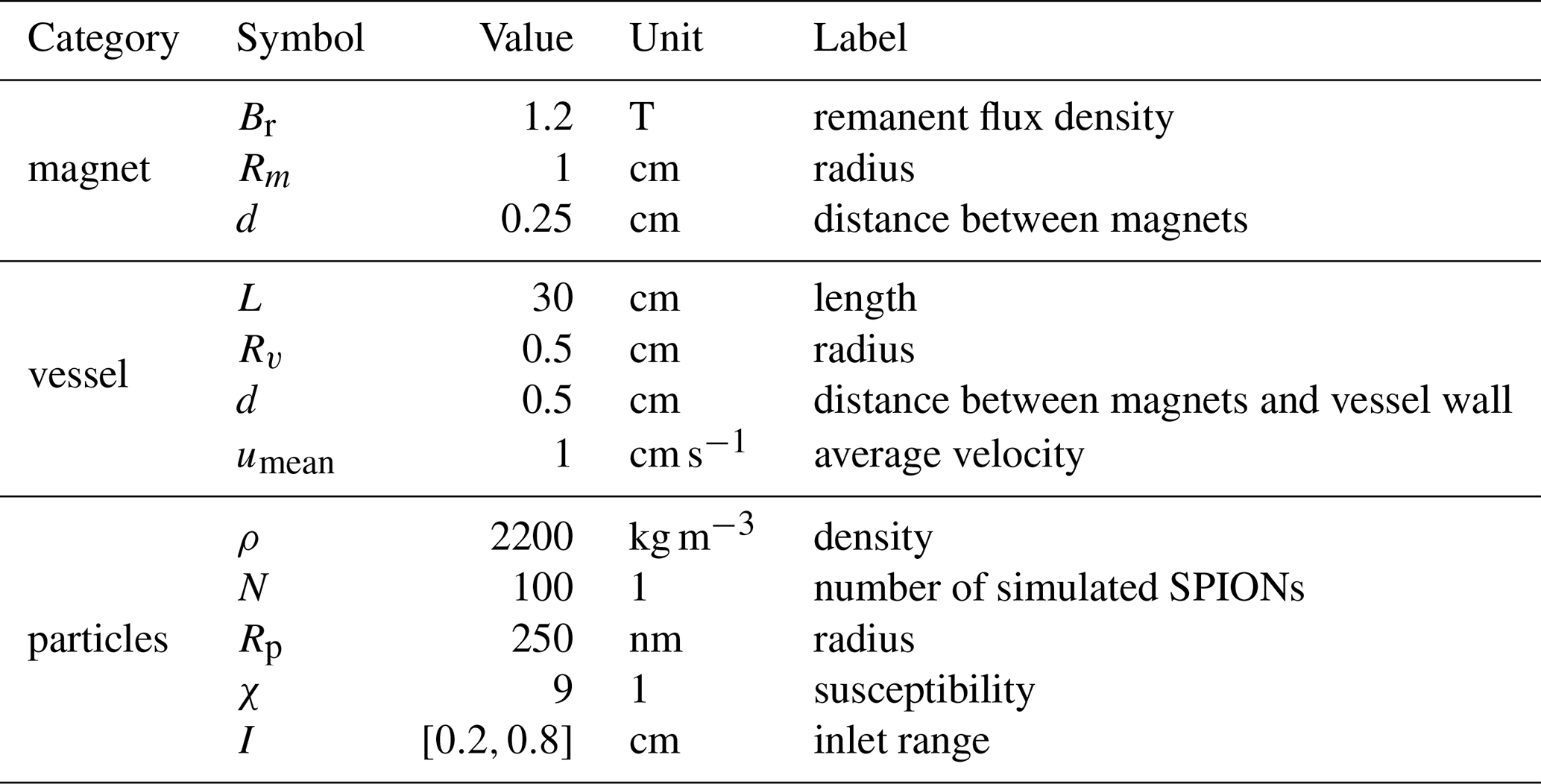
To investigate the performance of the particle steering, the linear Halbach array and the extended Halbach array were built up as a 2D model in COMSOL Multiphysics^® 5.6. Each array consists of 8 circular magnets and a Y-shaped geometry with a 30^∘ bifurcation representing the vessel. The setup is depicted in Fig. 3. In the simulations, the “Magnetic Fields, No Currents (mfnc)”, “Laminar Flow (spf)” and the “Particle Tracing (fpt)” modules were used. The fixed simulation parameters are summarized in Table 1. Here, the applied magnetic parameters correspond to typical values for NdFeB, whereas the fluid was set to water. In case of the adjustable Halbach array, the magnetization direction can be rotated over φ as shown in Fig. 1. Here, the magnetic field and the distribution of the SPIONs were investigated for discrete values with a step of $\mathit{\pi }/\mathrm{20}$, whereas in case of the extended Halbach array only the strong and the weak side as depicted in Fig. 2 were investigated. The magnetic flux density was studied at the three positions “1”–“3” in detail, which are denoted in red in Fig. 3.

Table 1 Fixed simulation parameters.

3 Results and discussion

In this section the simulation results will be presented and discussed. At first, the magnetic flux density of the different Halbach arrays at the three aforementioned evaluation positions will be investigated in detail. Afterwards, their performance on deflecting the SPIONs in the given scenario will be evaluated. For further investigating the magnetic force F_mag on the SPIONs, the gradient of the magnetic flux density has to be derived. In this work, this is done by fitting the simulation results of B for every x-position with the two fitting functions and determining the analytical derivative afterwards. The errors of the two fitting functions will be compared and the gradient of B evaluated. Finally, the magnetic force F_mag and the drag force F_drag will be investigated in detail and limitations of the proposed work will be explained.

3.1 Evaluation of the magnetic flux density

In Fig. 4, the isolines of the magnetic flux density B of the adjustable Halbach array are depicted for $\mathit{\phi }=\left[\mathrm{0},\mathit{\pi }/\mathrm{4},\mathit{\pi }/\mathrm{2}\right]$. It can be observed, that the Halbach array has a strong and a weak magnetic side, which can be switched by rotating φ from 0 to $\mathit{\pi }/\mathrm{2}$. The maximum value of the magnetic flux density B is the strongest for $\mathit{\phi }=\mathit{\pi }/\mathrm{4}$ and the weakest for φ=0 and $\mathit{\pi }/\mathrm{2}$. The maximum values are located between the first and second (or last and second last) magnet as can be seen in Fig. 4. However, the maximum flux densities differ only in 0.04 T. Furthermore, for φ=0, B is approx. constant in the x-direction in the region of the vessel, whereas for $\mathit{\phi }=\mathit{\pi }/\mathrm{4}$, the magnetic flux density is symmetric on both sides of the array.

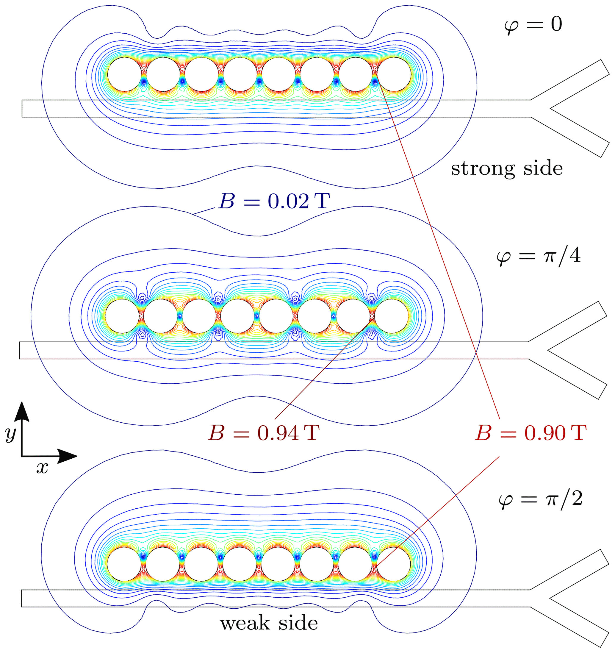
Figure 4 Isolines of the magnetic flux density B of the adjustable Halbach array for various rotation angles φ (Reprinted with permission from Thalmayer et al., 2021; © IEEE).

In Fig. 5, the isolines of the magnetic flux density B for the weak and the strong side of the extended Halbach array are illustrated. Here, the maximum value of the flux density is slightly increased compared to the adjustable Halbach array and is located between the second and third (or third and second last) magnet. However, in comparison to the field of Fig. 4, the flux density is not that compact and also less homogeneous in x-direction.

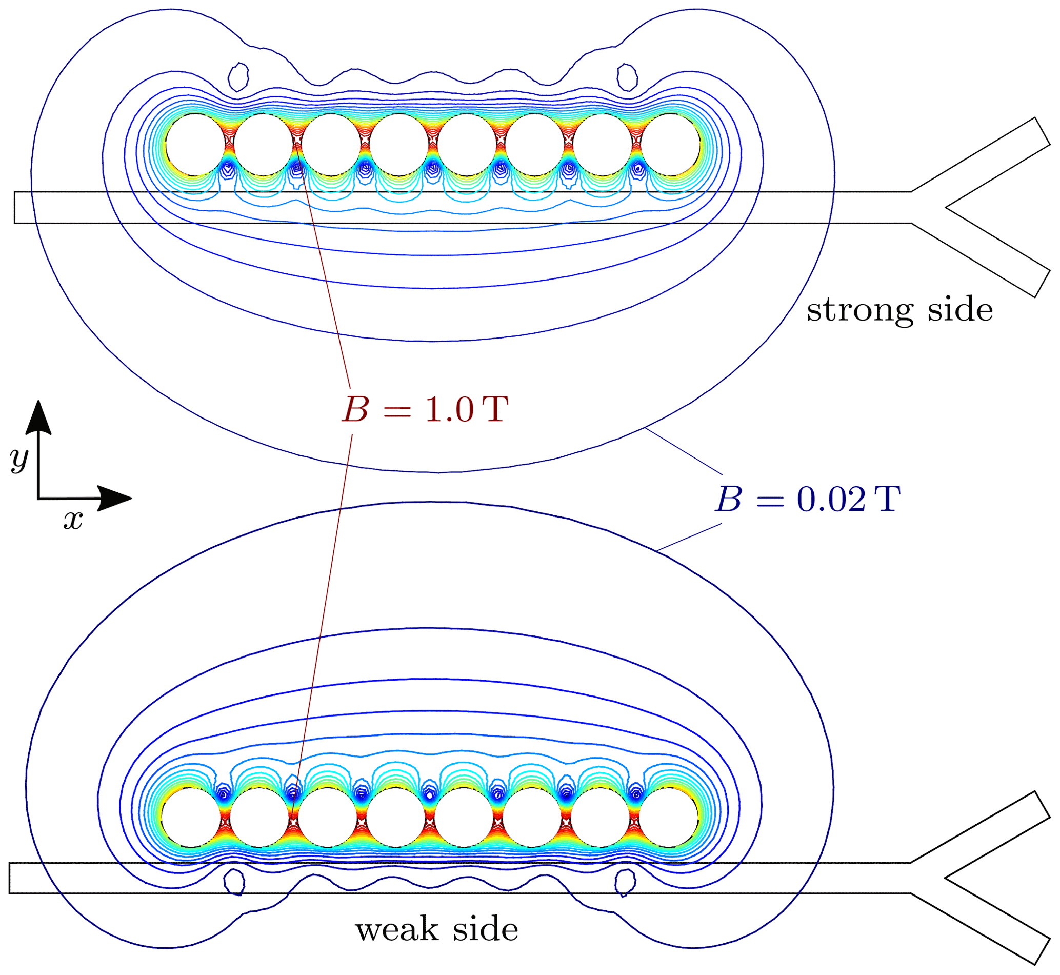
Figure 5 Isolines of the magnetic flux density B for the strong and the weak side of the extended Halbach array.

The variation of B(y) along the x-direction is evaluated by computing its standard deviation (std) for every y inside the vessel over the length beneath the magnets for φ=0 and $\mathit{\phi }=\mathit{\pi }/\mathrm{2}$ for the adjustable and for the strong and weak side for the extended Halbach array, respectively. In case of the adjustable Halbach array, for both φ, the std is by a factor of 10 smaller than the average value of B. However, the most significant changes occur at the outer magnets. Thus, the std is evaluated excluding the area under the two outer magnets, resulting in a std being 50 times smaller than the mean B. Similar results were archived for the extended Halbach array. However, here the std was only approximately a factor of 5 (full length) and 20 (excluding outer magnets) smaller. By decreasing the angle between the magnetization direction of two adjacent magnets even more, the results become worse. Thus, it can be seen, that the magnetic field is more homogeneous for the adjustable Halbach array with a magnetization shift of 90^∘ between two neighboring magnets. Further investigations show, that the more magnets are used and the smaller the distance d between the magnets is, the more homogeneous is B. However, this results in drawbacks, namely more needed space and a stronger torque. Thus, the number of magnets and d is restricted to 8 and 0.25 cm, respectively.

The behavior of the magnetic flux density B at the three evaluation positions, is illustrated in Fig. 6. Both, the adjustable and the extended Halbach array, for φ=0 and $\mathit{\phi }=\mathit{\pi }/\mathrm{2}$ and the strong and weak side are analyzed, respectively. Directly at the magnets, the flux density is approximately in the same magnitude for both arrays, however, B decays faster for the weak magnetic sides. At the distance of 0.5 cm, where the vessel starts, B is approx. 3 times greater for the strong side compared to the weak side. Overall, it can be seen that for the strong side (φ=0) and for the weak side ($\mathit{\phi }=\mathit{\pi }/\mathrm{2}$) the magnetic flux density is stronger for the adjustable Halbach. Moreover, the results in Fig. 6 depict, that B is stronger at positions underneath the magnets (position 1 and 3). Nevertheless, apart from position 2 at the strong side of the arrays, B decays for all functions approx. exponentially with the distance from the magnets.

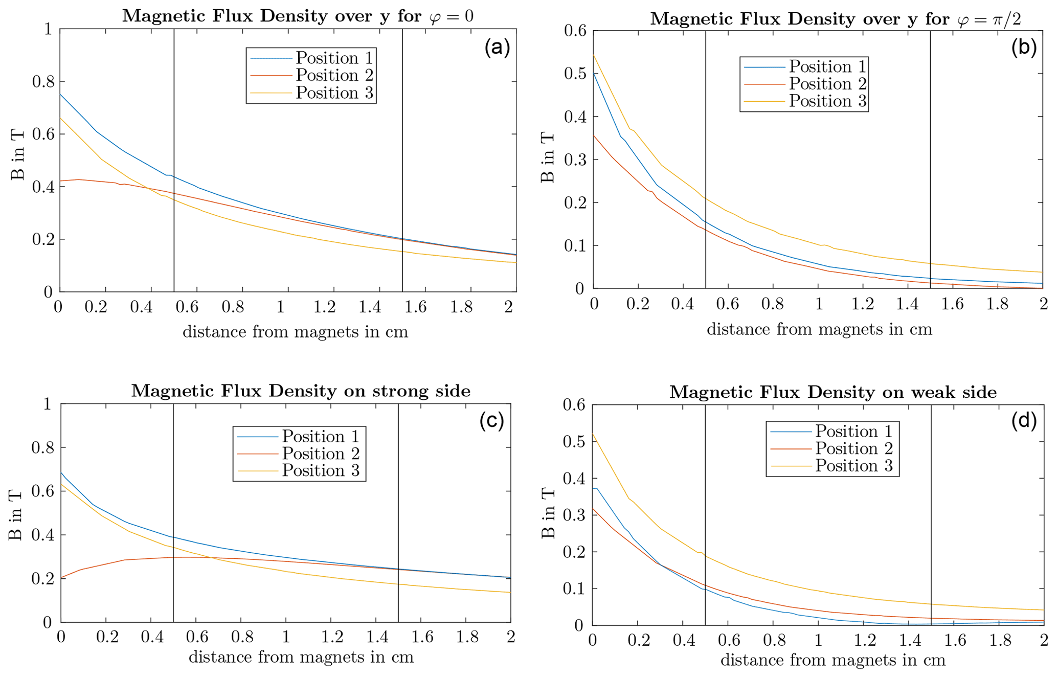
Figure 6 Magnetic flux density B over y for the different evaluation positions for φ=0 and $\mathit{\phi }=\mathit{\pi }/\mathrm{2}$ of the adjustable Halbach array (a, b) and for the strong and weak magnetic side of the extended Halbach array (c, d). The black vertical lines corresponds to the vessel walls.

3.2 Evaluation of SPION distribution

For the adjustable Halbach array, the propagation of the SPIONs for a fixed rotation angle φ of the magnetization direction was investigated. The distribution of the SPIONs to the branches is depicted in Fig. 7.

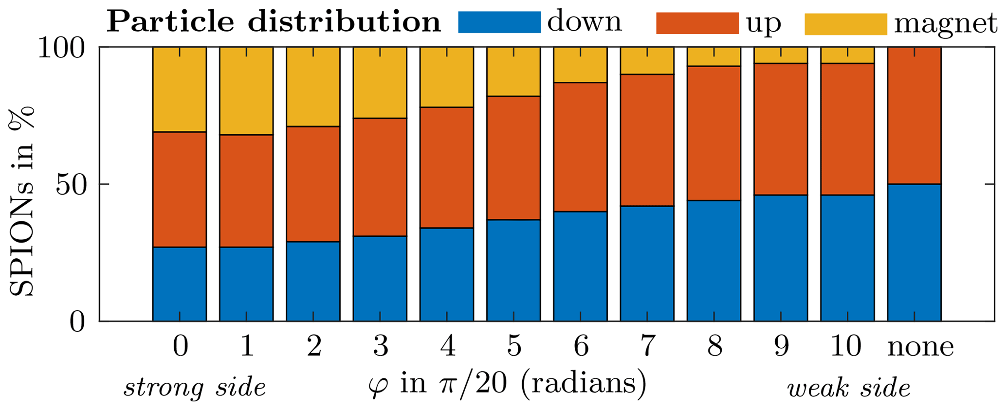
Figure 7 Distribution of the SPIONs for different rotation angles φ of the magnetization direction for the adjustable Halbach array. The blue and the red color correspond to the SPIONs taking the lower and upper branch, respectively; yellow represents the number of SPIONs trapped by the magnets. For the case “none”, no magnet was considered in the simulation (Reprinted with permission from Thalmayer et al., 2021; © IEEE).

Without the magnet (labeled “none” in Fig. 7), the SPIONs split equally between the upper and lower branch. With the Halbach array, Fig. 7 depicts that for the strong side of the array (φ=0), only 27 % of the SPIONs are in the lower branch. However, 31 % of the SPIONs get trapped by the magnet and, thus, remain in the vessel. For the weak side ($\mathit{\phi }=\mathit{\pi }/\mathrm{2}$), 46 % of the SPIONs are in the lower branch, while 6 % get trapped.

For the extended Halbach array (not plotted in Fig. 7) in case of the strong side 49 %, 37 % and 14 % take the upper, lower branch and get trapped by the magnet, respectively. In case of the weak side facing the vessel, 52 % and 48 % of the SPIONs take the upper and lower branch, respectively. Overall, it can be seen that the influence of the magnetic field on the SPIONs is stronger for the adjustable Halbach array. The reason can be found in the homogeneity of the magnetic field and its strong gradient as described in the section before. This leads to a strong and approximately constant magnetic force over a large area all underneath the magnets, resulting in a significant effect on the particles.

3.3 Evaluation of the gradient and fitting of the magnetic flux density

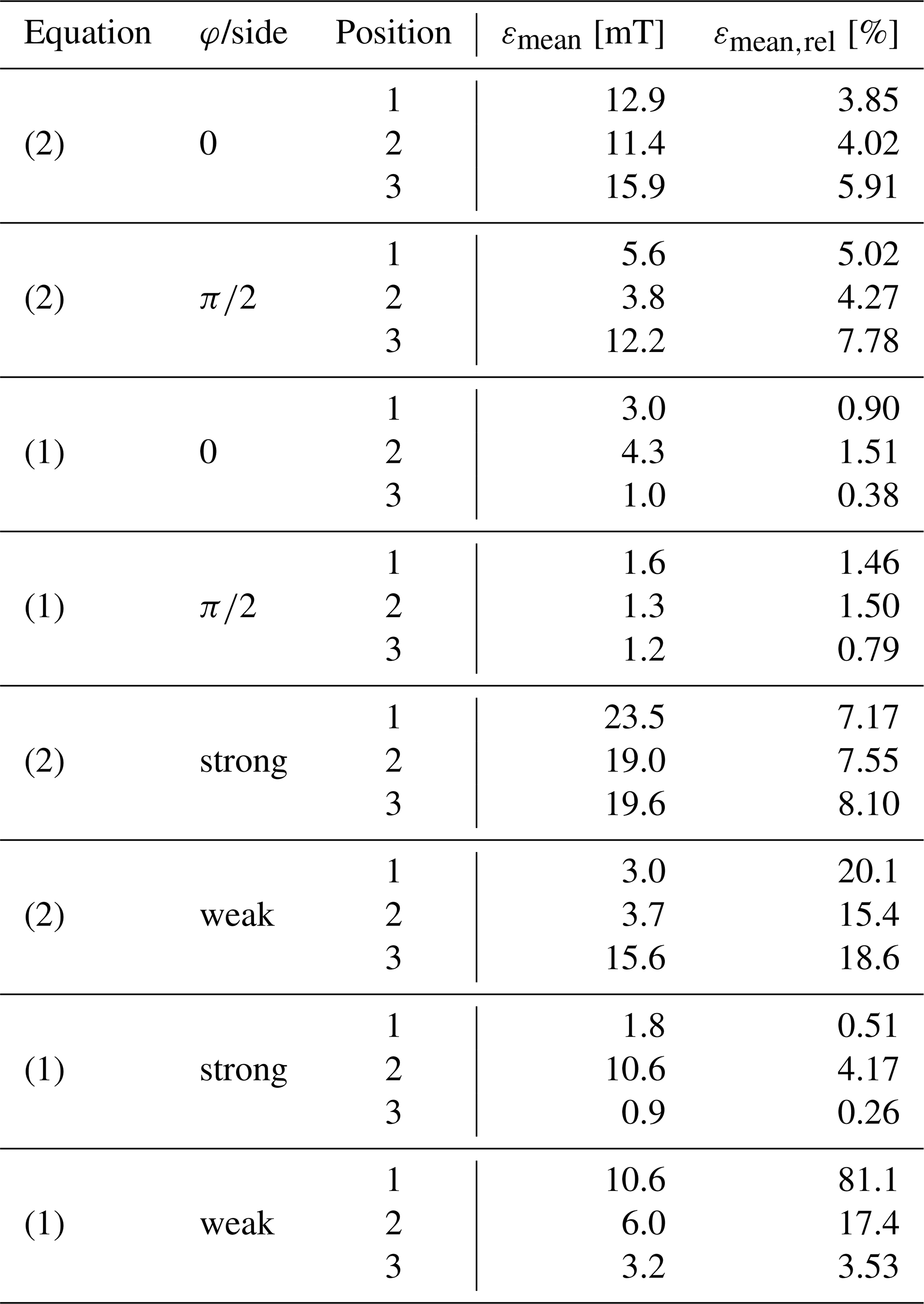
Since B is calculated numerically on a mesh in Comsol, the numerical calculation of the gradient of B is quite challenging. Thus, by determining the derivative, there are a lot of irregularities and additional noise on it. Therefore, in this work, the derivative is determined analytically using the results of the fitting functions (Eqs. 1 and 2). The mean fitting error for both equations and both arrays is summarized in Table 2. More detailed tables are listed in Appendix A.

Table 2 Comparison of the mean fitting errors of the the exponential Eq. (2) and the analytic Eq. (1) function for different rotation angles φ for the adjustable Halbach array and for the strong and weak side of the extended Halbach array.

Overall, the fitting performs quite well for both functions over the whole evaluation domain. By considering only the results inside the vessel, the errors even decrease, since the greatest errors occur directly at the boundary of the magnets. The fitting errors are smaller for the analytic fitting function Eq. (1). However, this is obvious, since six arbitrary constants are used in contrast to the exponential fitting function where only two were considered. In general, the fitting results perform better for the adjustable Halbach array than for the extended one. Furthermore, the errors are smaller for the strong side of the adjustable and extended Halbach array. This can especially be seen in the relative errors. The reason can be found in the magnitude of the magnetic field: for the strong side small errors result in smaller relative errors than for the weak side. Additionally, due to the numerical calculation on the mesh of B, there are discretization errors in the solution (compare Fig. 6). Since the fitting errors were conducted by subtraction the fitted results from the simulated one, this discretization can lead to high (especially relative) fitting errors.

Applying the fitting functions, the gradient of B can be determined. Since the exponential approach (Eq. 2) and it derivative are less complex and perform sufficient enough, it is used in the following. The resulting gradients for both Halbach arrays are depicted in Fig. 8. The gradient directly next to the magnet is stronger for the two weaker sides of the arrays. However, the gradient decreases very fast there, whereas the gradient of the two strong sides stays high over a larger distance. Moreover, the gradient is stronger directly under the magnets (positions “1” and “3”) and, therefore, the magnetic force on the particles is also stronger.

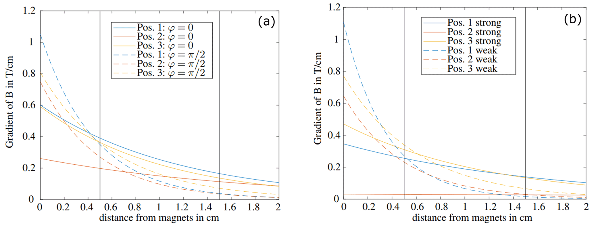
Figure 8 Gradient of the magnetic flux density B for the different evaluation positions of the adjustable Halbach array (a) and the extended Halbach array (b). The solid lines correspond to φ=0 and the strong side and the dashed lines to $\mathit{\phi }=\mathit{\pi }/\mathrm{2}$ and the weak side of the extended Halbach array, respectively.

3.4 Evaluation of F_mag and F_drag

To steer the particles, the main idea is to attract the SPIONs by a strong magnetic field and then rotate the array to get the particles washed out by the (hydrodynamic) drag force F_drag. For this purpose, the magnetic force F_mag and F_drag are calculated underneath the magnets. F_drag reaches values from 0 N at the boundary to $\mathrm{9.4}\cdot {\mathrm{10}}^{-\mathrm{11}}$ N at the center of the vessel. Before F_mag can be investigated at every position of the vessel, M of the particles has to be determined first. This is done by evaluating F_mag,y and the gradient G of the magnetic flux density at a fixed position in the simulation. From Eq. (4) and with $F_{\mathrm{mag},y}=\mathrm{8.38}\cdot {\mathrm{10}}^{-\mathrm{13}}$ N and G=32 T m⁻¹, M is calculated to $M\approx \mathrm{4}\cdot {\mathrm{10}}^{\mathrm{5}}$ A m⁻¹. This is in good accordance to the results of Alexiou et al. (2006) and Wei and Wang (2018). For reasons of simplification, the magnetization is assumed to be constant. Based on this, F_mag reached values from $\mathrm{5.1}\cdot {\mathrm{10}}^{-\mathrm{14}}$ to $\mathrm{2.1}\cdot {\mathrm{10}}^{-\mathrm{12}}$ N in the area underneath the magnets. The strongest and weakest F_mag was calculated for φ=0 and $\mathit{\phi }=\mathit{\pi }/\mathrm{2}$, respectively.

Additionally, F_mag,max and F_mag,mean were calculated for both arrays. Furthermore, the ratio $F_{\mathrm{d}-\mathrm{m}}=F_{\mathrm{drag}}/F_{\mathrm{mag}}$ is evaluated for every x and y. The results are listed in Table 3. F_d−m has a minimum of 0, since F_drag=0 N at the vessel wall, and maximum values of 236 and 647 for the adjustable Halbach array, respectively. For φ=0, F_d−m is smaller, since F_mag on the SPIONs is stronger in this case. For the extended Halbach array, the ratio is even greater (608 and 1454), illustrating that the magnetic force on the particles is much smaller for this array.

Table 3 Comparison of the results for different rotation angles φ for the adjustable Halbach array and for the strong and weak side of the extended Halbach array.

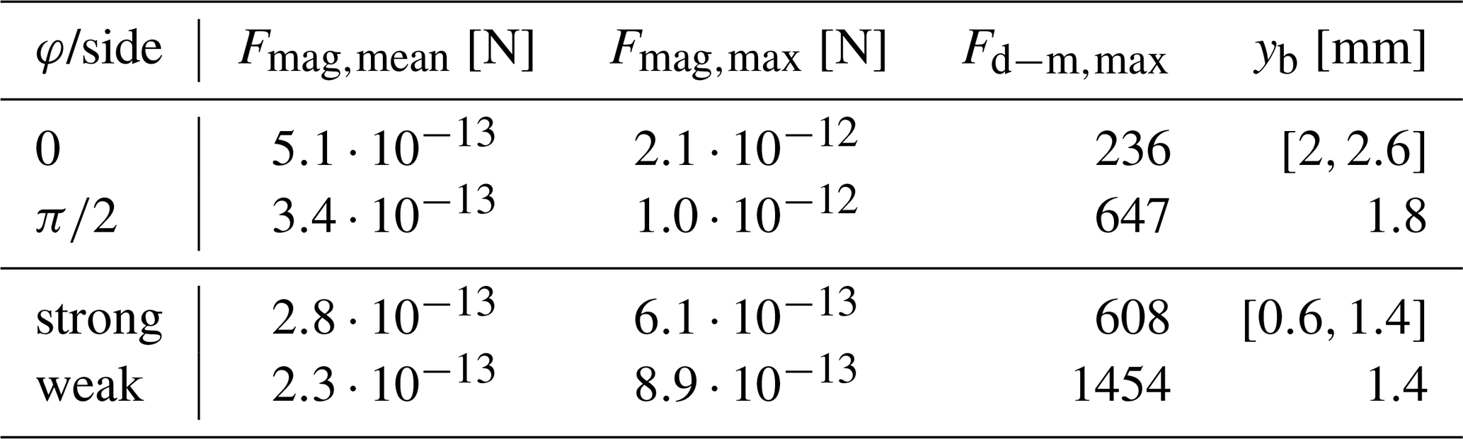
Besides, the main moving direction is given by F_d−m. At a ratio of >100, the influence of the magnetic force on the SPIONs is assumed to be negligible. For this, a boundary distance y_b [m] was calculated, which corresponds to the distance from the upper vessel for $F_{\mathrm{d}-\mathrm{m}}\le \mathrm{100}$ (see Table 3). The ratio F_d−m is also illustrated in Fig. 9 exemplary for the strong and the weak side of the adjustable Halbach array. To make the boundary y_b visible, F_d−m is set equal to 0 for all values <100.

Figure 9 Ratio of ${\mathit{F}}_{\mathrm{drag}}/{\mathit{F}}_{\mathrm{mag}}$ of the adjustable Halbach arry. For ratios smaller than 100, the ratio is set to 0 to make the boundary y_b visible.

As expected, y_b is greater for φ=0. For $\mathit{\phi }=\mathit{\pi }/\mathrm{2}$, the boundary distance is quite constant, whereas in the results of φ=0 the inhomogeneity of B can be seen. The minima and maxima have a distance of 2.25 cm, which corresponds to the distance of the magnets in the array. This is in good accordance with the results of the gradient (compare Fig. 8), which is predominantly underneath the magnets. Moreover, the adjustable Halbach array also performs better than the extended Halbach array, since y_b is smaller, which fits also to the results of the gradient.

3.5 Limitations of this study

It is worth mentioning, that the proposed study has some limitations: Within the simulations, the particles were considered separately. This means, that the interaction between the particles among each other were neglected. Also the change of the magnetic field due to the particles propagating through it, is not taken into account. Furthermore, the magnetization within the SPIONs is assumed to be constant. However, it can be observed from measurements that the particles form chains parallel to the magnetic field lines (Myrovali et al., 2021). This changes the magnetic field distribution and, therefore, the magnetic force on the particles.

Moreover, for the magnetic force F_mag only the component in the y-direction is taken into account, since B is dominant in this direction. However, of course B has a component and gradient in the x-direction, too. The particles are accelerated before one magnet of the array and decelerated after it. Furthermore, this also contributes to agglomeration of the particles directly underneath the magnets, which again changes the magnetic field distribution.

Another limitation of this study is caused by the permanent magnets. They cannot be switched off like an electromagnet. Therefore, there will be always a remaining magnetic field and, thus, a magnetic force towards the magnets, even for the weak side. In consequence, the magnetic array has to have a certain distance to the vessel, which, however, results in the decrease of the magnetic force for the strong side.

4 Conclusions

In this extended paper, an adjustable linear Halbach array and an extended version for steering magnetic nanoparticles were investigated numerically by using COMSOL Multiphysics^®. Both Halbach arrays provide a strong and a weak magnetic side, which can be switched by rotating the single magnets. In case of the adjustable Halbach array, this can be done by a simultaneous rotation of all single magnets around 90^∘ clockwise or counterclockwise, respectively, whereas in case of the extended array the switching is much more complex. The magnetic field, its gradient and the force on magnetic particles were analyzed for different rotation angles of the magnets as well as for the strong and weak magnetic side of the extended Halbach array. For the calculation of the gradient, two different fitting functions were compared.

The results reveal that overall the adjustable Halbach array performs better than the extended one in both, changing the magnetic force easily and deflecting the particles. In general it can be concluded that the magnetic force is the strongest directly underneath the magnets and by rotating the single magnets, the region where the drag force is able to wash the particles out, can be adjusted. In future research, the simulation model will be expanded and every second magnet of the adjustable Halbach array will be replaced by an electromagnet. Therefore, the configuration has to be optimized to design a proper electromagnet needing less space and power. By that, the strong and weak magnetic side can be switched by switching the direction of the current. With this, an electromagnetic field of travelling waves similar to a linear motor drive will be designed for steering the particles to a desired region.

Appendix A: Fitting Errors

The errors for the fitting of the magnetic flux density with the exponential Eq. (2) and the analytic Eq. (1) are listed in detail in Table A1 for the adjustable Halbach array and in Table A2 for the extended Halbach array, respectively.

Table A1 Overview of the fitting results for the exponential Eq. (2) and the analytic Eq. (1) for the different evaluation positions of the adjustable Halbach array. All absolute fitting errors ε are given in mT and the relative ones (in brackets) in %. For the last two columns, only the results inside the vessel were considered.

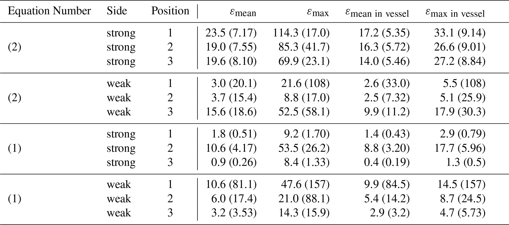
Table A2 Overview of the fitting results for the exponential Eq. (2) and the analytic Eq. (1) for the different evaluation positions of the extended Halbach array. All absolute fitting errors ε are given in mT and the relative ones (in brackets) in %. For the last two columns, only the results inside the vessel were considered.