 | 10 Dec 2020
Scattering and diffraction of a uniform complex-source beam by a slit in a perfectly conducting plane screen
Ludger Klinkenbusch
A new multipole solution in plane-polar coordinates for the scattering of an arbitrary TE- or TM-polarized incident field by an infinitely extended slit in a plane screen is derived. To this end a classical three-domain problem with a complete multipole expansion in each of the domains is formulated. The unknown multipole amplitudes are found from the continuity conditions of the tangential electric and magnetic field components. Finally an infinite system of linear equations is derived which can be approximated by a numerically tractable finite one leading to a solution with an arbitrary accuracy. The results are numerically successfully compared to those ones obtained by classically solving the strip problem using Mathieu functions and by a subsequent application of the rigorous form of the Babinet principle. Numerical results include the comparison of the scattered fields obtained for an incident uniform complex-source beam and for an incident plane wave.
- Article
(8803 KB) - Full-text XML
- BibTeX
- EndNote


Because of its general theoretical and practical interest the scattering and diffraction of acoustic and electromagnetic waves by a slit has been very often discussed in the literature. An early contribution to that subject was given by Schwarzschild (1902) who proposed an approximate method based on the famous half-plane solution derived by Sommerfeld (1896). Later, Sieger (1908) introduced a solution for the strip in elliptic cylinder coordinates where this geometry can be described by a coordinate surface as a flattened elliptic cylinder. The corresponding solution of the Helmholtz equation for the strip problem is based on Mathieu functions. According to the rigorous form of the Babinet principle (Bouwkamp, 1954) the field diffracted by a slit can be exactly deduced from the field diffracted by a strip. Morse and Rubinstein (1938) used this method and computed first numerical results for the scattering of TM- and TE-polarized plane waves by a strip/slit. Many other contributions on that subject have been published since then including works on the asymptotic evaluation using GTD/UTD techniques (Suedan and Jull, 1987). An overview on methods and results on that subject can be found in Bowman et al. (1998).
In the present work we introduce an alternative method to exactly solve the slit/strip problem (Klinkenbusch, 2019). We formulate a three-domain boundary-value problem in plane-polar coordinates. In each of the domains we constitute a complete multipole ansatz consisting of products of Bessel or Hankel functions with harmonic functions. The modified incident field in this formulation is build from the classical incident field (which would exist in the free space) plus the field reflected from the plane. The multipole amplitudes are analytically found from the continuity conditions of the tangential electric and magnetic field components at the boundaries between the domains and from suitably applied orthogonality relations. The special definition of a modified incident field leads to identical results for the scattered fields above and below the plane which allows to state a system of linear equations with the scattered-field amplitudes as the unknowns.
The numerical evaluation includes a successful validation of the method by comparing the results with those obtained by the aforementioned solution of the strip problem and application of the Babinet principle. Then we compare the scattered fields for an incident plane wave to those obtained for an incident uniform complex-source beam with different parameters. The goal of this investigation is to find out if and for which parameters a uniform CSB can replace an incident plane wave. This can be useful for many applications – particularly in the context of scattering from special sections as part of infinitely extended structures like the scattering by the tip of a circular or elliptic cone.
Consider the geometry in Fig. 1. A perfectly electrically conducting (PEC) plane at y=0 is broken by a slit (width 2R0) symmetrically located around the z-axis. We introduce cylindrical coordinates with x=Rcos φ; y=Rsin φ. We are looking for a rigorous solution of the TMz case where the phasor of the incident electric field intensity is given by , and of the TEz case where the phasor of the incident magnetic field intensity is described by . denotes the unit vector in z-direction. Here and in the following a phasor is defined with respect to a time-factor exp {+jωt} with and ω representing the angular frequency.
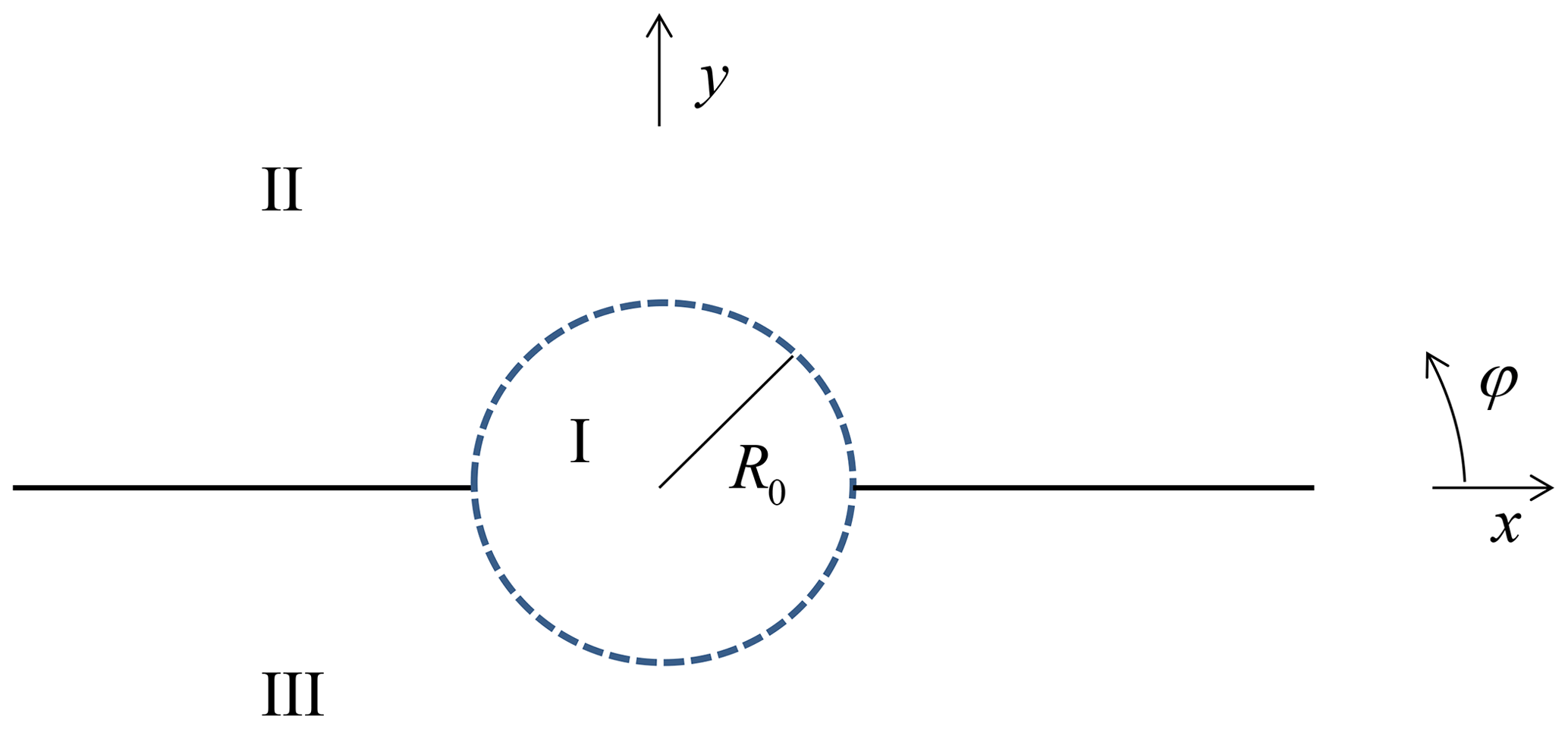
We split the entire space into three domains as sketched in Fig. 1. Domain I consists of a circular-cylindrical domain with radius R0 centered at the z-axis while the domains II and III are defined by and , respectively. In domain II we split the total field into a known incident part (index inc) and into a scattered part (index sc).
2.1 Solution of the TMz problem
In each of the domains I, II, and III we introduce a complete plane-polar multipole expansion for the electric field intensity according to:
Here, is the wave number with the permittivity ε and permeability μ, Jn and represent Bessel functions of the first kind and Hankel functions of the second kind to satisfy regularity at R=0 as well and to comply with the Sommerfeld radiation condition, respectively. Note that is defined as an arbitrary incident field in domain II in the presence of the conducting plane at y=0, i.e., it includes the corresponding reflected field.
The Hφ-component of the magnetic field follows from Faraday's law according to:
Note that the multipole amplitudes of the incident field are known. For finding the other multipole coefficients and we have to consider the boundary- and continuity conditions of the electromagnetic field.
At the circular boundary around domain I the tangential components of the electric field intensity have to be continuous:
We insert Eqs. (1)–(5) into Eq. (11), multiply the result by cos (mφ), integrate on the interval (0,2π), and finally obtain while using the orthogonality of the harmonic functions:
In Eq. (13) the Neumann number is given by
while the scalar products are defined according to:
Next, multiplying Eq. (11) by sin (mφ) and integrating on leads to:
Now we insert Eqs. (6)–(10) into Eq. (12), multiply the result by cos (mφ) and sin (mφ), respectively, integrate on the interval (0,2π), and obtain
and
respectively. Combining Eq. (18) with Eq. (13) and Eq. (19) with Eq. (17) leads to:
and
respectively. As easily can be shown it holds:
From Eqs. (22) and (21) it immediately follows that
which reflects the symmetry of the scattered field originating from the slit in the domains II and III. With Eqs. (24) and (23) we write Eq. (20) as
which approximately can be written as a finite system of linear equations to determine the from the :
The elements of the checkerboard-like matrix in Eq. (26) are found as
while for the elements of the right-hand side we obtain:
For a quadratic system of linear equations in Eq. (26) we choose for the upper limits and . Finally, with Eq. (24) we conclude from Eqs. (22) and (17)
while Eq. (13) yields:
2.2 Solution of the TEz problem
In each of the domains I, II, and III we introduce a complete plane-polar multipole expansion for the magnetic field intensity and according to:
Again the incident field is defined as the field of an arbitrary source in domain II in the presence of the perfectly electrically conducting plane at y=0, i.e., it includes the reflected field.
The φ-component of the corresponding electric field follows from Maxwell's law according to:
At the boundary to domain I, the tangential fields have to be continuous:
A similar procedure as in the TMz case leads to a finite system of linear equations to determine the from the :
The elements of the checkerboard-like matrix are found as
while for the elements of the right-hand side we have:
To obtain a quadratic system of linear equations we choose for the upper limits and . Finally, the multipole amplitudes in the domains III and I are found as
and
respectively.
2.3 Scattered far fields
In domain III, the scattered far-field can be obtained from Eq. (5) or from Eq. (35) using the asymptotic expression of the Hankel function of the second kind for large values of its argument:
The electric far-field reads for the TMz case
while the magnetic far field for the TEz case is obtained as:
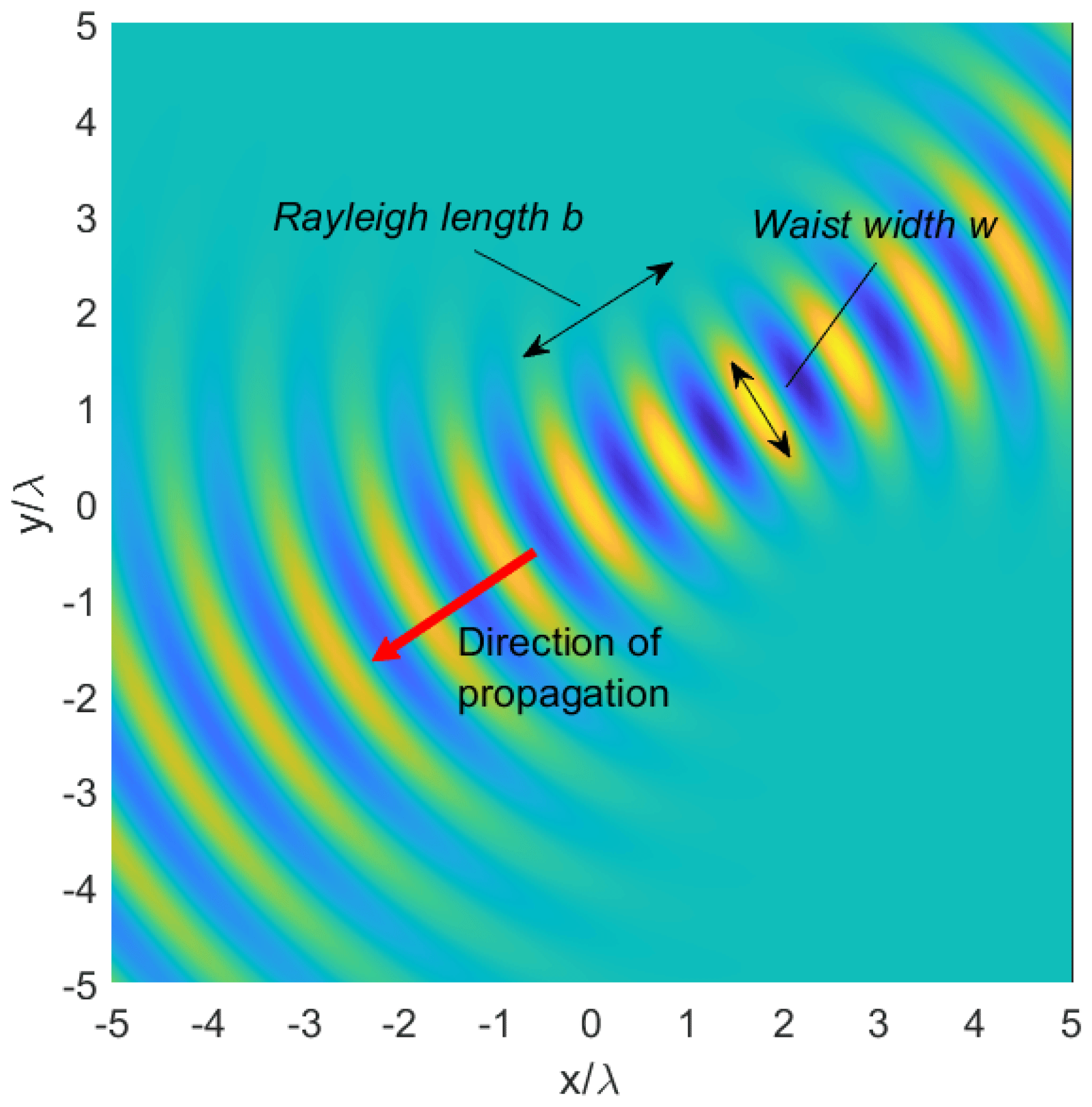
Figure 2 Snapshot of a uniform CSB with . The beam width of the waist is characterized by . The focus length is b.
A complex-source beam (CSB) is obtained for a complex-valued point-source coordinate. As has been shown, in a paraxial approximation a CSB represents a Gaussian beam (Felsen, 1976). More specifically, for the present two-dimensional problems the multipole amplitudes of a CSB which is propagating from the waist directly towards the origin (i.e., the z-axis) are found to be (Katsav et al., 2012)
for the TMz- and TEz-case, respectively. In Eqs. (51) and (52), the radial coordinate is defined by
where E0 and H0 are the amplitudes, Rinc,φinc represent the location of the waist of the CSB, and b is the focus (or Rayleigh) length. It can be shown (Felsen, 1976) that the analogy between a CSB and a Gaussian beam is valid nearby the axis (par-axial) and only on that side of the waist from which the field is propagating away. Moreover, as can be seen from the behaviour of the Hankel function directly in the waist the field of the CSB is not regular. On the other hand, by choosing Hankel functions of the first kind (instead of second kind) in Eqs. (51) and (52) we obtain a par-axial Gaussian beam approximation on the other side of the waist which is travelling towards the waist. By adding both CSBs one obtains a par-axial approximation of a complete Gaussian beam which moreover is regular everywhere including the waist (uniform CSB). Similar to (Klinkenbusch and Brüns, 2016) where the proof has been outlined for the 3D case for the present case the multipole amplitudes for an incident uniform CSB can be found as:
Figure 2 shows a snap-shot of a uniform CSB and the relation of b to the parameter of the corresponding Gaussian beam.
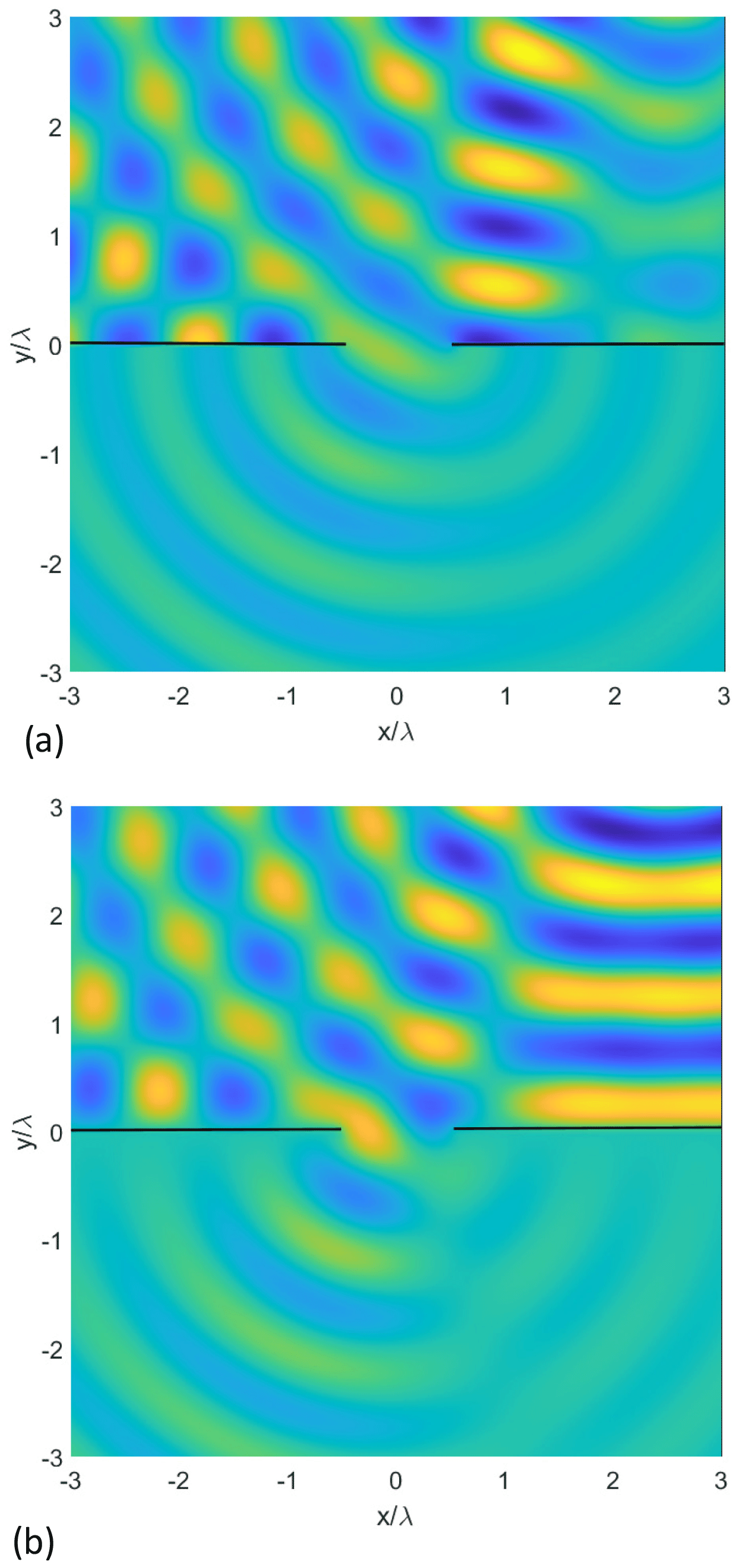
Figure 3 Snapshots of the near fields obtained by the present approach using 60 eigenfunctions for the incident field, 40 eigenfunctions for the scattered field in regions II and III, and 20 eigenfunctions in region I. (a) TMz-case and (b) TEz-case. Lines sources at Rinc=5λ, . Width of the slit: 1λ.
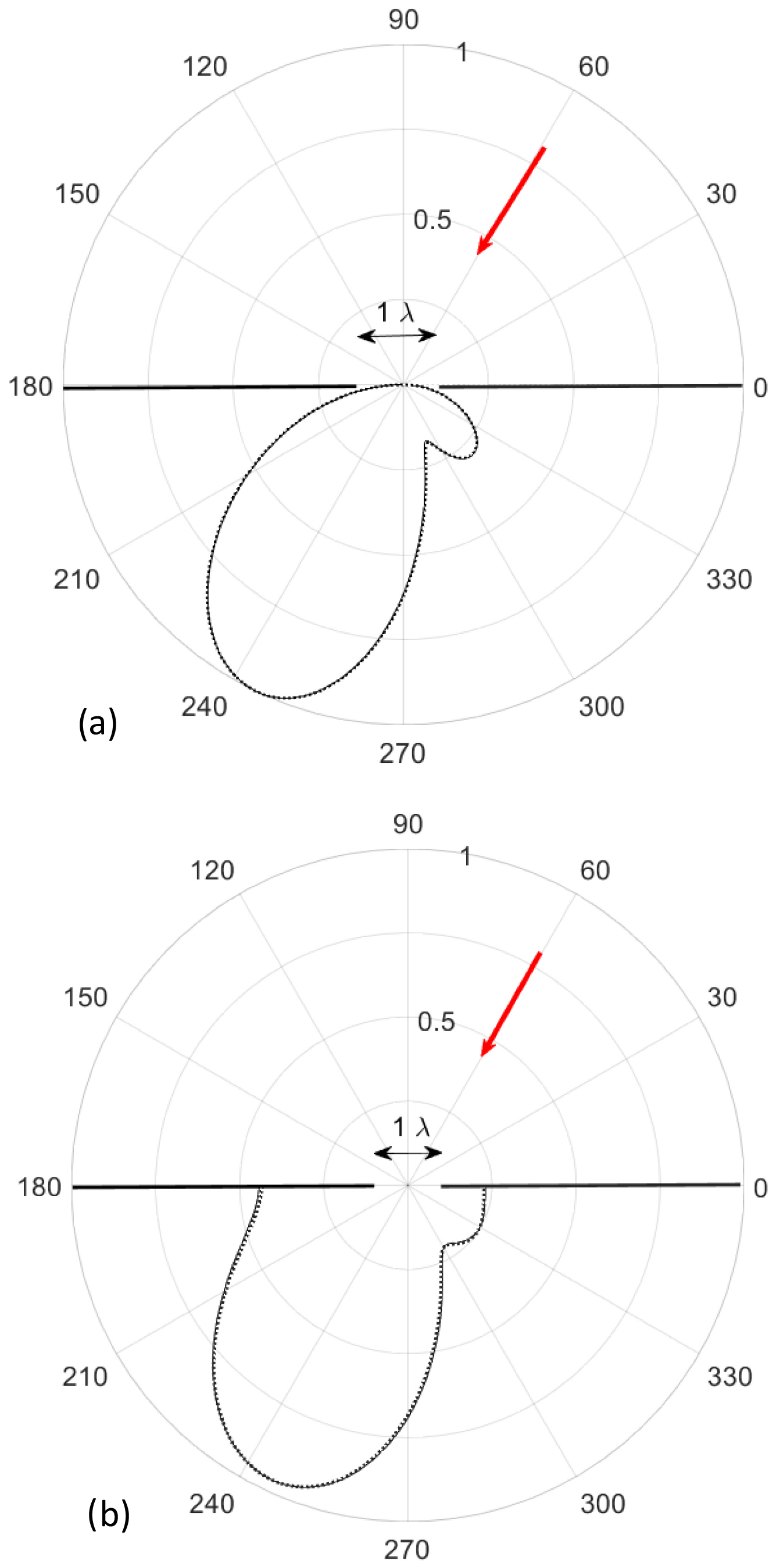
Figure 4 Comparison between the normalized far fields obtained by the present approach using 40 eigenfunctions (solid) for the scattered field and by applying the rigorous form of Babinet principle to the solution found for the strip in elliptic coordinates using 8 eigenfunctions, i.e. products of radial and angular Mathieu functions (dotted). (a) TMz-case and (b) TEz-case. Lines sources at Rinc=5λ, . Width of the PEC slit/strip: 1λ.
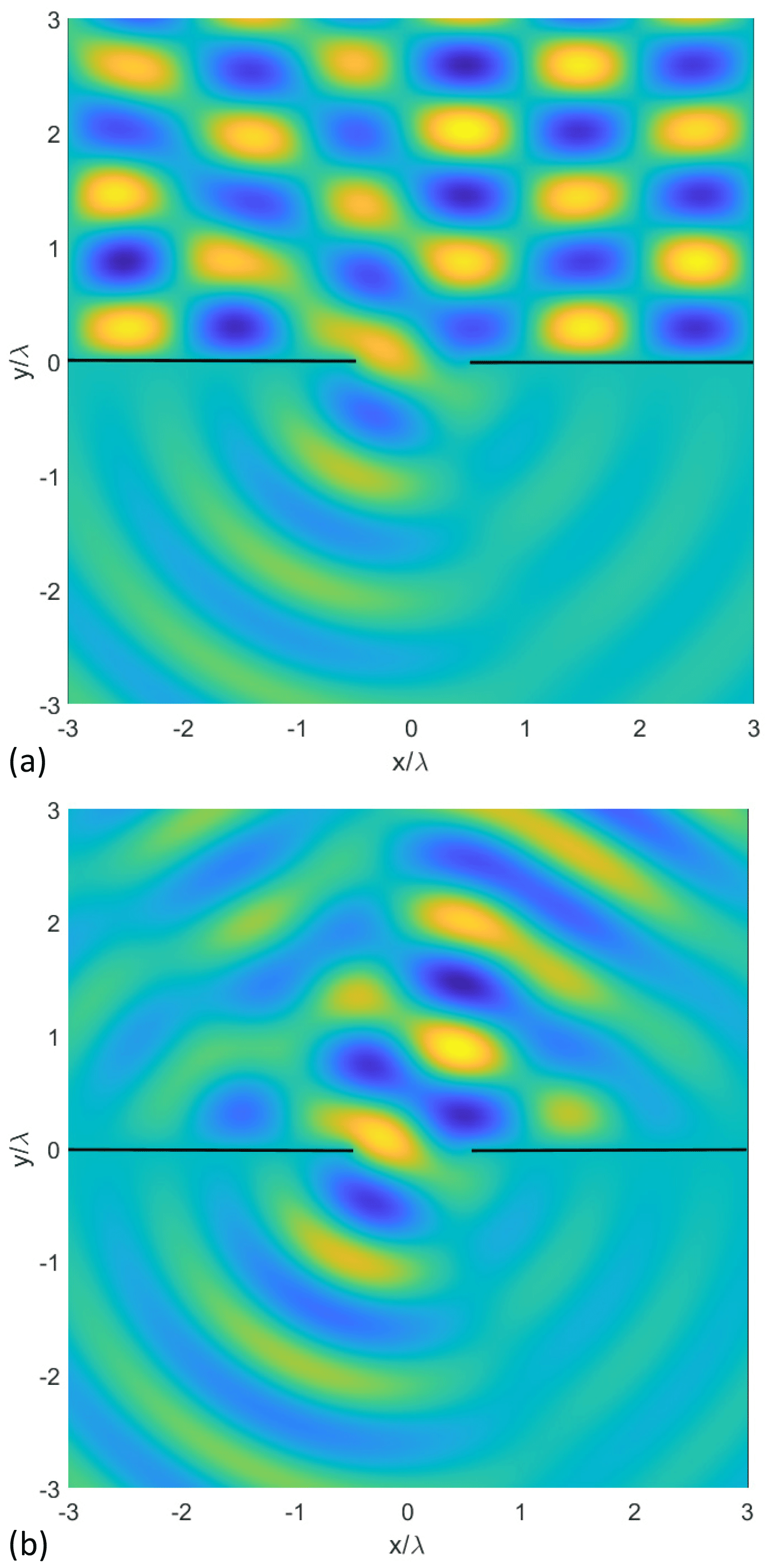
Figure 5 Snapshots of the TMz-polarized near fields (a) for an incident plane wave, and b) for an incident uniform CSB. Waist centered at Rinc=0.001λ, . Width of the slit: 1λ. Focus length: b=5λ. 60 eigenfunctions for the incident field, 40 eigenfunctions for the scattered field in regions II and III, and 20 eigenfunctions in region I.
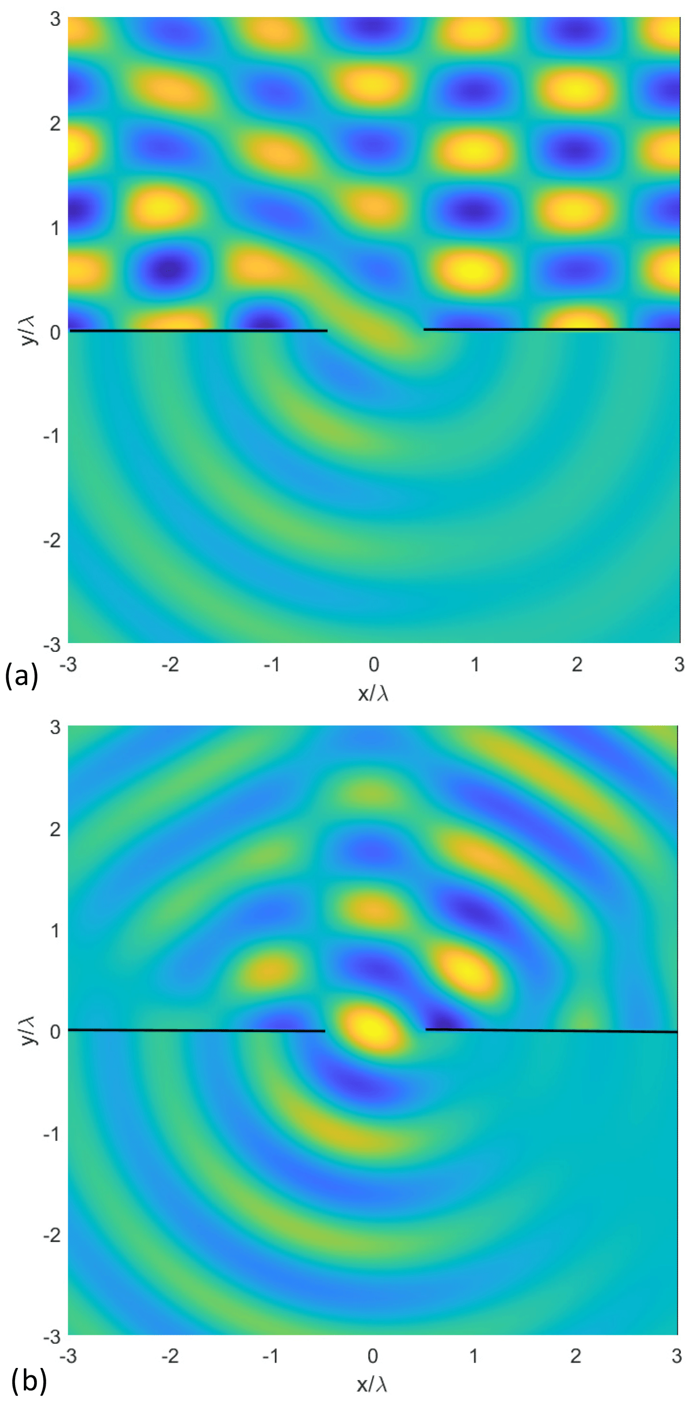
Figure 6 Snapshots of the TEz-polarized near fields (a) for an incident plane wave, and (b) for an incident uniform CSB. The other data are the same as in Fig. 5.
4.1 Convergence properties
Basically, all of the infinite series involved for solving the boundary value problem have to be truncated to come to a numerical solution. The maximal order of multipole functions needed for a desired accuracy of the scattered field (for instance, nmax in Eqs. 4 and 5) depends on the electric size of the scatterer. More quantitatively this follows from the behavior of Bessel functions of the first kind with half of the electric width of the slit (κR0) as the argument. As has been outlined in Chew et al. (1998, p. 51), a maximum order of with C being a positive number which directly corresponds the number of relevant digits is a suitable choice to obtain an accurate far-field. Moreover, mmax must be larger than nmax in Eqs. (28) and (29) hence the following rule for the number of eigenfunctions applies:
4.2 Validation
We start with a comparison of the results of the current approach to those ones obtained by solving the complementary problem of a strip using Mathieu functions and a subsequent application of the rigorous form of the Babinet principle (Bouwkamp, 1954). All numerical results have been obtained using MATLAB© including a toolbox for the numerical calculation of the Mathieu functions (Cojocaru, 2020). Figure 3 show snapshots of the diffracted (total) near fields in case of a line source located at . Note that identical results are obtained in both cases if the fields are calculated by applying the classical method, i.e., by solving the strip problem using Mathieu functions with 8 eigenfunctions and a successive application of the rigorous form of the Babinet principle. The CPU time on an AMD Ryzen 3700 platform needed for calculating the field at 100×100 points is 69.70 s for the classical method using Mathieu functions and 1.15 s for the present approach.
Figures 4 reveal that the scattered far-fields computed with the present and the classical approach are in an excellent agreement for both cases, TEz and TMz.
Finally we remark that the code used for the calculation of the Mathieu functions (Cojocaru, 2020) does not give sufficient information about its accuracy and consequently this validation is limited to a qualitative level.
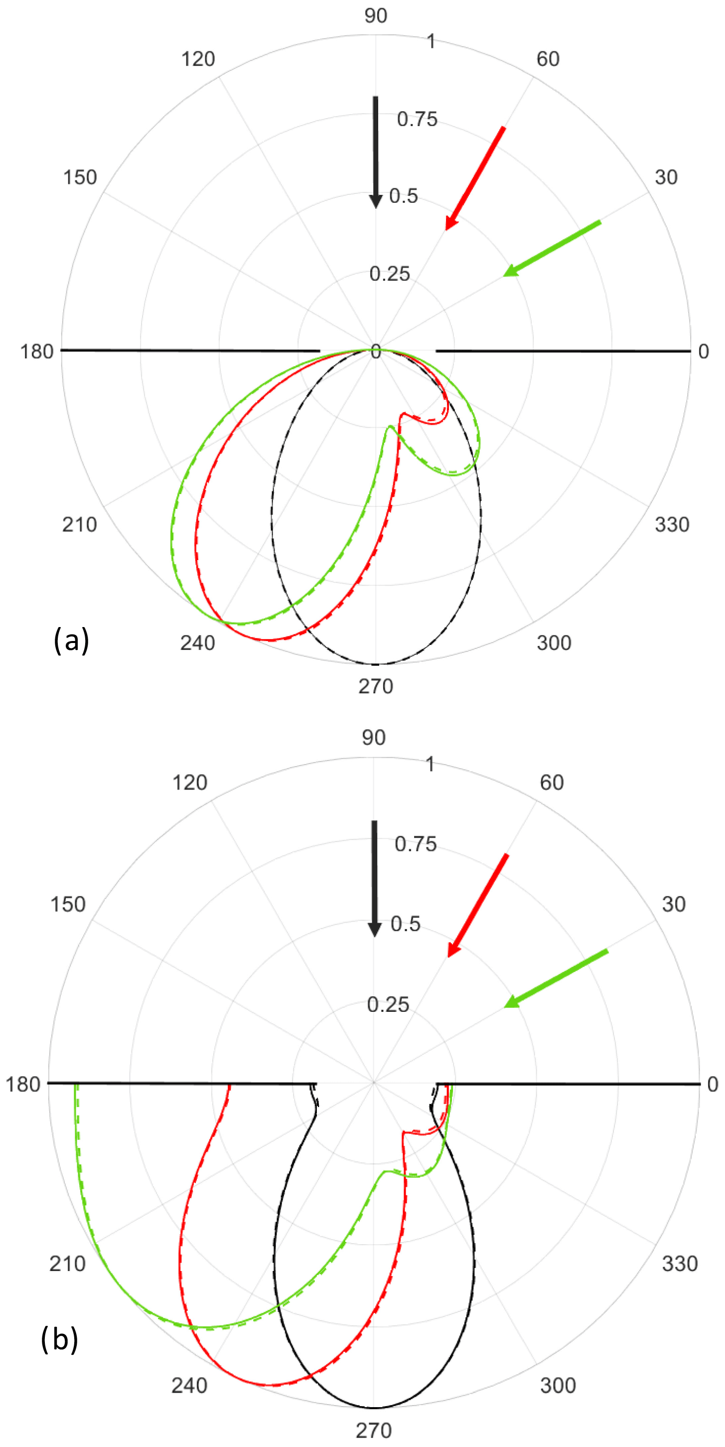
Figure 8 Polar diagrams of the scattered far-fields for an incident plane wave and for incident uniform CSBs with different values of the angle of incidence. (a) TMz-polarization; (b) TEz-polarization. The other data are the same as in Fig. 5.
4.3 Comparison between an incident uniform CSB and a plane wave.
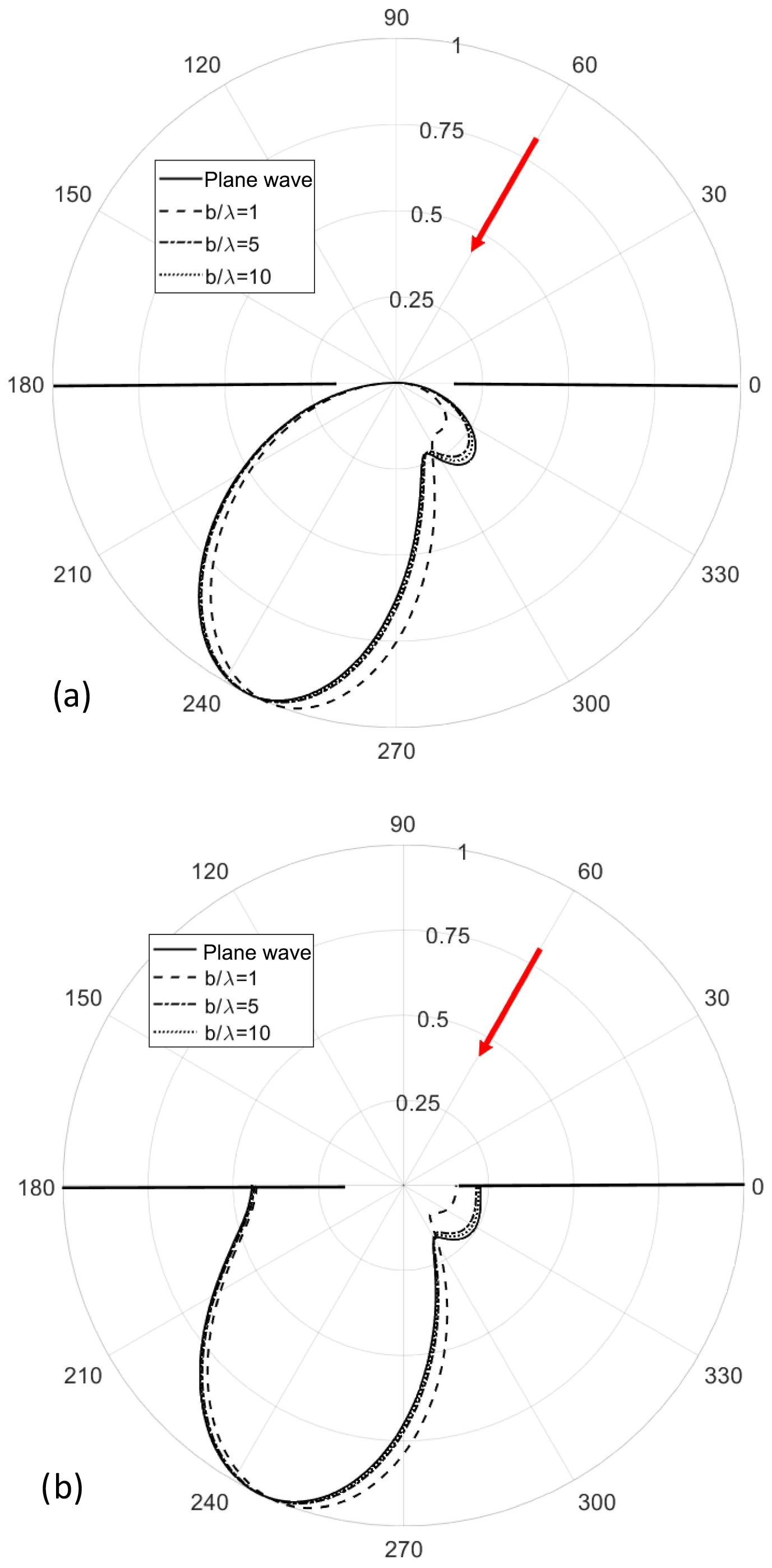
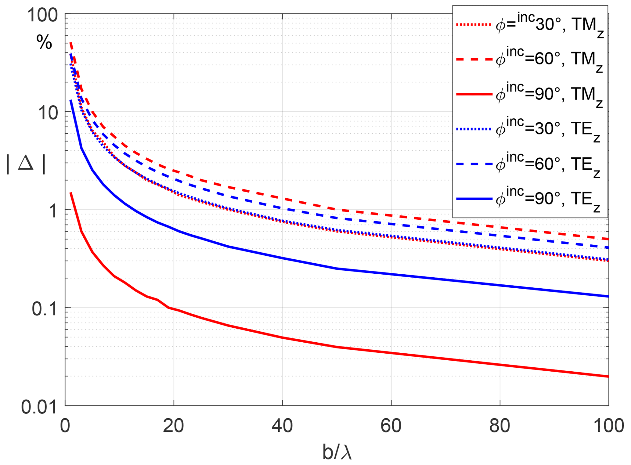
As described above the proposed solution can be easily extended to include the case of an incident uniform CSB. Of particular interest is the question whether a CSB can replace a plane wave to investigate the scattering by certain areas of a scattering object. As the best similarity of a uniform CSB to a localized plane wave is obviously in the waist, we choose its location almost at the center of the slit (Rinc=0.001λ). Figures 5 and 6 each show snapshots of the near-fields for an incident plane wave and for an incident uniform CSB in the TMz and TEz-polarization cases, respectively. The fields for an incident plane wave in the upper half plane each are dominated by the typical interference patterns and look completely different to those ones obtained for incident uniform CSB. In the lower half plane the results for an incident plane wave and for a uniform CSB each look similar. More quantitatively, Fig. 7 represent the scattered far-fields for an incident plane wave compared to incident uniform CSBs with different values of the focus length b. The scattered far-fields obtained for an incident plane wave and for an incident uniform CSB are nearly identical except of a small deviations in the area of the side lobe. These deviations are larger for a smaller value of the focus length b because the width of the waist (where the uniform CSB represents a plane wave) is given by and thus getting smaller for smaller values of b. However, even for larger values of b the results do not perfectly agree to those ones obtained for an incident plane wave. The reason for this might be the fact that only the plane-wave equivalence is valid only at the center of the slit where the waist is located. At the other parts of the slit particularly at the edges the CSB represents a converging or a diverging field. Consequently for a symmetrically incident uniform CSB (see Fig. 8) there is the best agreement between the scattered fields for both cases, incident plane wave and incident uniform CSB. More quantitatively, Fig. 9 represents the relative maximum deviation between the scattered far fields for an incident plane wave (index pw) and an incident uniform CSB (index csb) for different values of the angle of incidence as a function of b∕λ. The relative maximum deviation regarding the TMz-case is defined by
The relative maximum deviation for the TEz-case is found by simply replacing the electric by the corresponding magnetic scattered far-fields in Eq. (57).
As expected, an increase of the focus length and corresponding beam width leads to a reduction of the maximum relative deviation. Moreover, for the TMz-case we observe a higher dependence of the maximum relative deviation on the angle of incidence than for the TEz-case.
A new direct method to analytically solve the electromagnetic scattering and diffraction by a slit has been derived. The results are in agreement to those ones obtained by the classical solution in elliptic coordinates using Mathieu functions and a subsequent application of the rigorous form of the Babinet principle. It has been shown that an incident uniform complex-source beam can be used instead of an incident plane wave if the waist is chosen to be located nearby the slit and the beam width at the waist has been chosen to be sufficiently larger than the slit.
The data are available from the author upon request.
The author declares that there is no conflict of interest.
This article is part of the special issue “Kleinheubacher Berichte 2019”. It is a result of the Kleinheubacher Berichte 2019, Miltenberg, Germany, 23–25 September 2019.
This paper was edited by Thomas Eibert and reviewed by two anonymous referees.
Bouwkamp, C. J.: Diffraction theory, Rep. Prog. Phys., 17, 35–100, 1954. a, b
Bowman, J. J., Senior, T. B. A., and Uslenghi, P. L. E. (Eds.): Electromagnetic and Acoustic Scattering by Simple Shapes (Revised Printing), Hemisphere Pub., New York, 1998. a
Chew, W. C., Jin, J.-M., Michielssen, E., and Song, J. (Eds.): Fast and Efficient Algorithms in Computational Electromagnetics, Artech House, Boston, Vol. 52, 2001. a
Cojocaru, E.: Mathieu Functions Toolbox v.1.0, available at: https://www.mathworks.com/matlabcentral/fileexchange/22081-mathieu-functions-toolbox-v-1-0, MATLAB Central File Exchange, last access: 22 February 2020. a, b
Felsen, L. B.: Complex-Source-Point Solutions of the Field Equations and Their Relation to the Propagation and Scattering of Gaussian Beams, in: Symposia Mathematica, Istituto Nazionale di Alta Matematica, London, UK, Academic, vol. XVIII, 40–56, 1976. a, b
Katsav, M., Heyman, E., and Klinkenbusch, L.: Scattering and Diffraction of a Complex-Source Beam by a Wedge, Proceedings of the 2012 IEEE International Symposium on Antennas and Propagation, https://doi.org/10.1109/APS.2012.6348778, 2012. a
Klinkenbusch, L.: Scattering and Diffraction of a Uniform Complex-Source Beam by a Slit, 2019 Kleinheubach Conference, Miltenberg, Germany, 2019. a
Klinkenbusch, L. and Brüns, H.: Combined Complex-Source Beam and Spherical-Multipole Analysis for the Electromagnetic Probing of Conical Structures, Compte Rendue Physique, 17, 960–965, 2016. a
Morse, P. M. and Rubenstein P. J.: The Diffraction of Waves by Ribbons and Slits, Phys. Rev., 54, 895–898, 1938. a
Schwarzschild, K.: Die Beugung und Polarisation des Lichts durch einen Spalt [The Diffraction and Polarization of Light by a Slit], Math. Ann., 55, 177–247, 1902 (in German). a
Sieger B.: Die Beugung einer ebenen elektrischen Welle an einem Schirm vom elliptischem Querschnitt [The Diffraction of a Plane Electric Wave by a Screen of Elliptic Cross Section], Ann. Phys., 27, 626–664, 1908. a
Sommerfeld, A.: Mathematische Theorie der Diffraction [Mathematical Theory of Diffraction], Math. Ann., 47, 317–74, 1896. a
Suedan, G. A. and Jull, E. V.: Two-Dimensional Beam Diffraction by a Half-Plane and Wide Slit, IEEE T. Antenn. Propa., 35, 1077–1083, 1987. a