 | 10 Dec 2020
Approximation and analysis of transient responses of a reverberation chamber by pulsed excitation
Konstantin Pasche
Fabian Ossevorth
Ralf T. Jacobs
Reverberation chambers show transient behaviour when excited with a pulsed signal. The field intensities can in this case be significantly higher than in steady state, which implies that a transient field can exceed predefined limits and render test results uncertain. Effects of excessive field intensities of short duration may get covered and not be observable in a statistical analysis of the field characteristics. In order to ensure that the signal reaches steady state, the duration of the pulse used to excite the chamber needs to be longer than the time constant of the chamber. Initial computations have shown that the pulse width should be about twice as long as the time constant of the chamber to ensure that steady state is reached. The signal is sampled in the time domain with a sampling frequency according to the Nyquist theorem. The bandwidth of the input signal is determined using spectral analysis. For a fixed stirrer position, the reverberation chamber, wires, connectors, and antennas can jointly be considered as a linear time-invariant system. In this article, a procedure will be presented to extract characteristic signal properties such as rise-time, transient overshoot and the mean value in steady state from the system response. The signal properties are determined by first computing the envelope of the sampled data using a Hilbert transform. Subsequent noise reduction is achieved applying a Savitzky–Golay filter. The point where steady state is reached is then computed from the slope of the envelope by utilising a cumulative histogram. The spectral analysis is not suitable to examine the transient behaviour and determine the time constants of the system. These constants are computed applying the method of Prony, which is based on the estimation of a number of parameters in a sum of exponential functions.
An alternative to the Prony Method is the Time-Domain Vector-Fit method. In contrast to the first mentioned variant, it is now also possible to determine the transfer function of the overall RC system. Differences and advantages of the methods will be discussed.
- Article
(4854 KB) - Full-text XML
- BibTeX
- EndNote


Reverberation Chambers are commonly used for immunity and emission tests, where an important class of immunity tests is performed with pulsed modulated sinusoidal signals. A reverberation chamber (RC) is characterised by its quality factor Q, which is dependent on the operating frequency f and the time constant τ of the chamber (Krauthäuser, 2007; Pfennig, 2015). The quality factor affects the time required until steady state is reached when the excitation is switched on. This characteristic places a limit on the minimum duration of the pulse with which the chamber can be excited if steady state is desired. Figure 1 shows a typical pulsed signal s with a sinusoidal carrier of frequency fc and magnitude A.
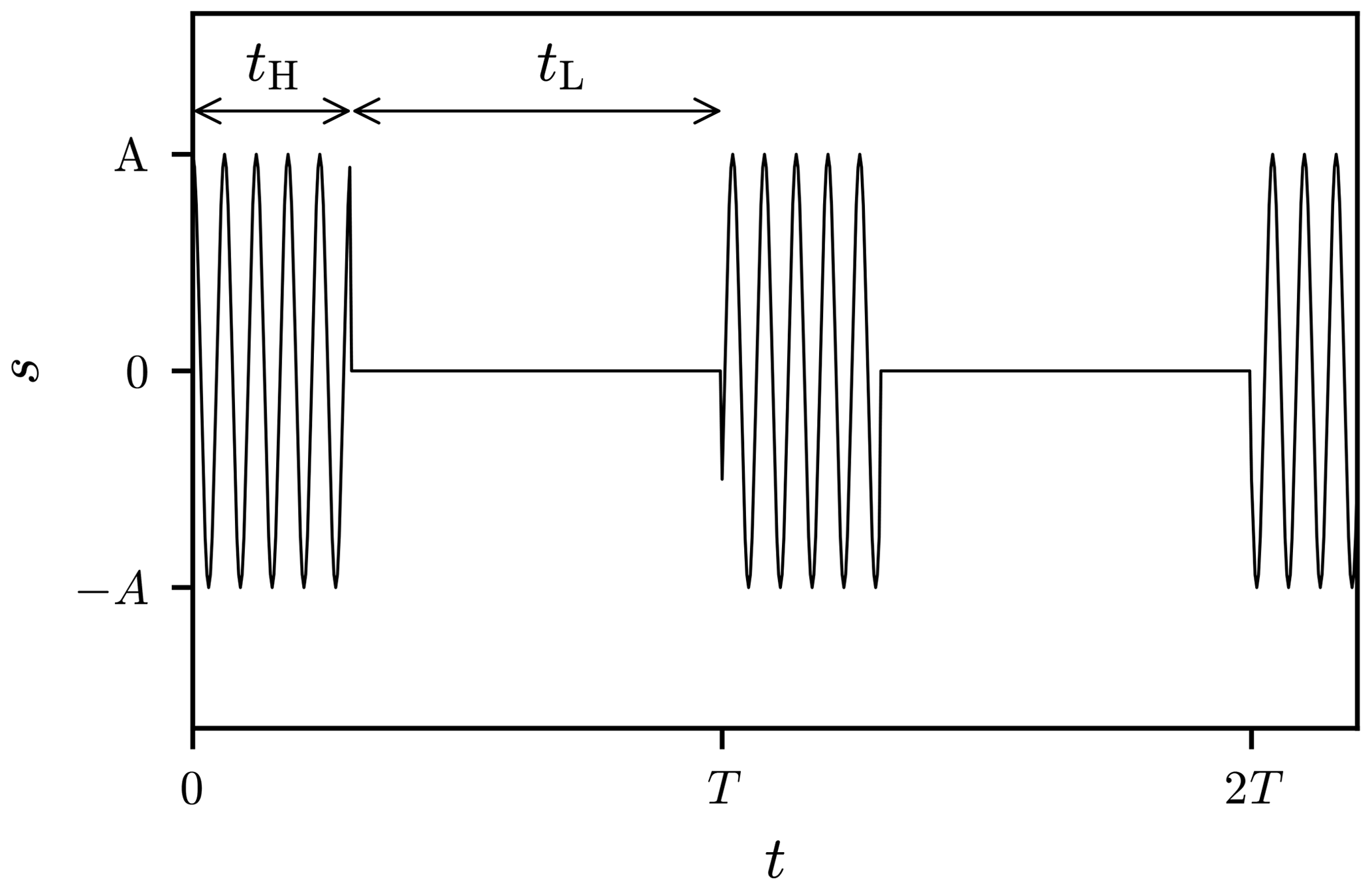
The duration of the pulse is denoted tH and the time between two pulses tL. The period T of the signal is, as a result, given by tH+tL. A typical value for the pulse duration is tH≥2.5τ, i.e. a multiple of the time constant (Deutsche Kommission Elektrotechnik Elektronik Informationstechnik im DIN und VDE, 2011). Transient behaviour is observable in the response of the RC if a switching event takes place. The field intensities can in this case be significantly higher than in steady state and possibly exceed predefined limits in an immunity test which consequently can damage the device under test (DUT).
A large number of publications have already dealt with transient behaviour in RCs (Artz, 2017; Manicke and Krauthäuser, 2012; Krauthäuser and Nitsch, 2002; Amador et al., 2010).
The possible overshoot can best be observed by measurements in time-domain. Artz has shown in his work that strong overshoot is accompanied by a low amplitude in the steady state and vice versa.
In contrast to the work of Artz (2017) it is not necessary to determine an ensemble mean value in advance of the evaluation. Each time series is evaluated individually.
The focus of this work is on signal analysis which depends on the stirrer position. First, in Sects. 2 and 3 a signal theoretical description of the overall RC system is given. The measurement setup and signal preprocessing is presented in Sect. 4.
An algorithm that extracts signal characteristics such as the amplitude of the overshoot when switching on and off as well as the amplitude at steady state is presented in Sect. 5.
The parameters thus obtained are required for further signal analysis.
The chamber response is recorded with an oscilloscope for each stirrer position and is therefore time-discrete. This time series of measurements is interpolated to a function that is continuous over time. The function depends on the location within the test volume, the time and the stirrer position.
In Sect. 6 the Method of Prony is used for this purpose. The transient behaviour of the RC exhibits exponential behaviour. By means of Prony's Method, which represents a sum of weighted exponential functions, this transient and decay behaviour can be represented intrinsically and is thus a well suited choice. For large data sets, the use of Prony's Method is not practical. This is due to the point wise nature of the method, where each data point is considered. A high time resolution and a long measurement duration result in large data sets, which leads to the problems mentioned above.
An alternative is the Time-Domain Vector-Fit method (Grivet-Talocia, 2004). Based on initial frequencies, a rational function is adapted to correspond to the measurement process in the time domain. An advantage over the Prony Method is the extraction of the transfer function of the entire system consisting of RC, antennas, cables and connectors. This procedure is presented in Sect. 7.
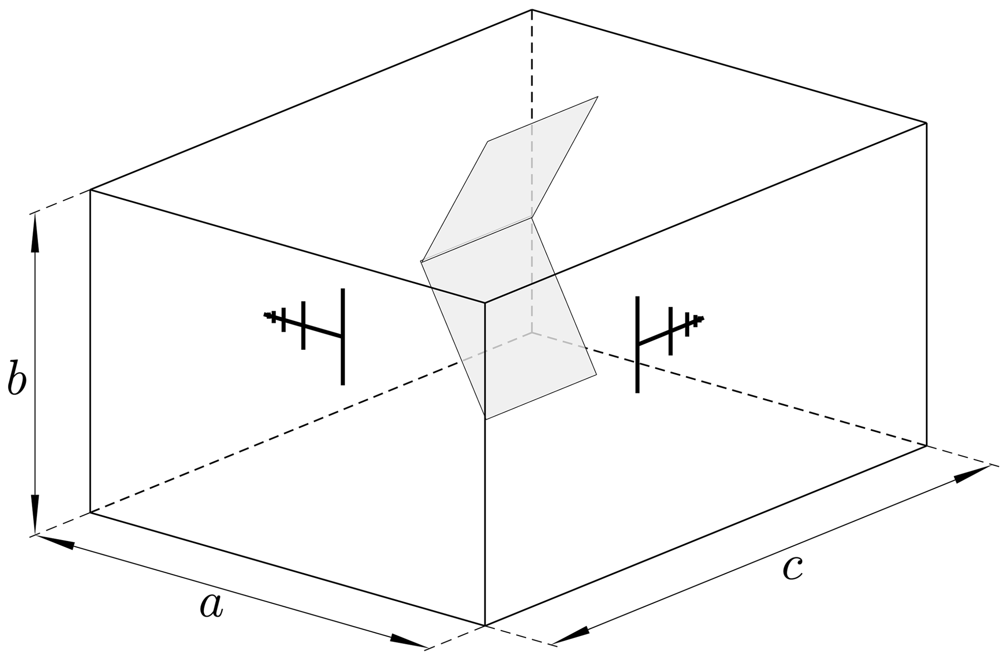
A typical RC which can be regarded as rectangular cavity of width a, height b, and length c, that is equipped with a mechanical stirrer, a transmitting and a receiving antenna is shown in Fig. 2.
Resonant cavities possess a linear time-invariant system and can therefore be considered as a linear time-invariant (LTI) system (Artz and Hirsch, 2014), as displayed in Fig. 3.
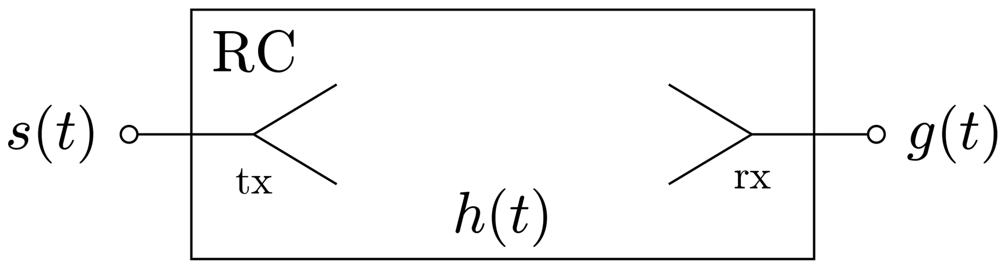
The system response g of the chamber,
is given by the convolution of the input signal s and the system impulse response h of the RC, where g, s and h are functions of time t. h can be determined by measurement (Artz and Hirsch, 2014). The system impulse response includes the impulse response of the receiving and transmitting antenna, cables and the feedthrough. LTI systems transform a time-harmonic input signal of a certain frequency to a time-harmonic output signal of the same frequency (Hoffmann, 1998). The resonant frequencies are determined by Hill (2009)
where μ denotes the permeability and ε the permittivity of medium in the RC. The indices m, n, p determine the field mode. A TE- and a TM-mode exists for every combination of m, n, and p unless one of the indices is zero. In this case, only a TE- or a TM-mode exists. Any equipment in the chamber changes the boundary conditions for the field and consequently affects the resonant frequencies so that modes are not known exactly.
To alleviate this problem an approximation of the mode density
can be used as a performance indicator for the RC, where c0 denotes the speed of light (Liu et al., 1983). Ds(f) provides information on the number of resonant frequencies in the neighbourhood of f. The mode density increases if the frequency increases. The chamber used for the measurements has a width a of 3.7 m, a height b of 3.0 m, a length c of 5.3 m, which amounts to a volume V of 58.83 m3. For a frequency of 400 MHz for example, the mode density Ds(f) in the given chamber equals 8.74 modes per MHz.
A key performance indicator of a RC is the quality factor Q, see Krauthäuser (2007).
A theoretical value for Q is given by
with the chamber volume V, the skin depth δS and the walls permeability μm. The skin depth of the wall material can be given as
with the wall conductivity σ.
A RC can electrically be viewed as a network of RLC circuits, see Bernard Demoulin (2011). Each excited mode can be modelled with an RLC circuit.
The signal displayed in Fig. 1 can be written as
where ωc=2πfc and φ represents the phase shift of the carrier at t=0 s. The rectangular function vanishes for t<0 s and t>tH, equals a half for t=0 s and t=tH, and equals one for . In order to generate a pulsed signal s, the single pulse is repeated periodically. The spectrum of the signal is determined by computing the Fourier coefficients
The identity
enables to rewrite s as
with
The frequency domain representation of is given by
and similarly
where the primed symbols refer to normalised variables, i.e.
The coefficients Sn can finally be written as
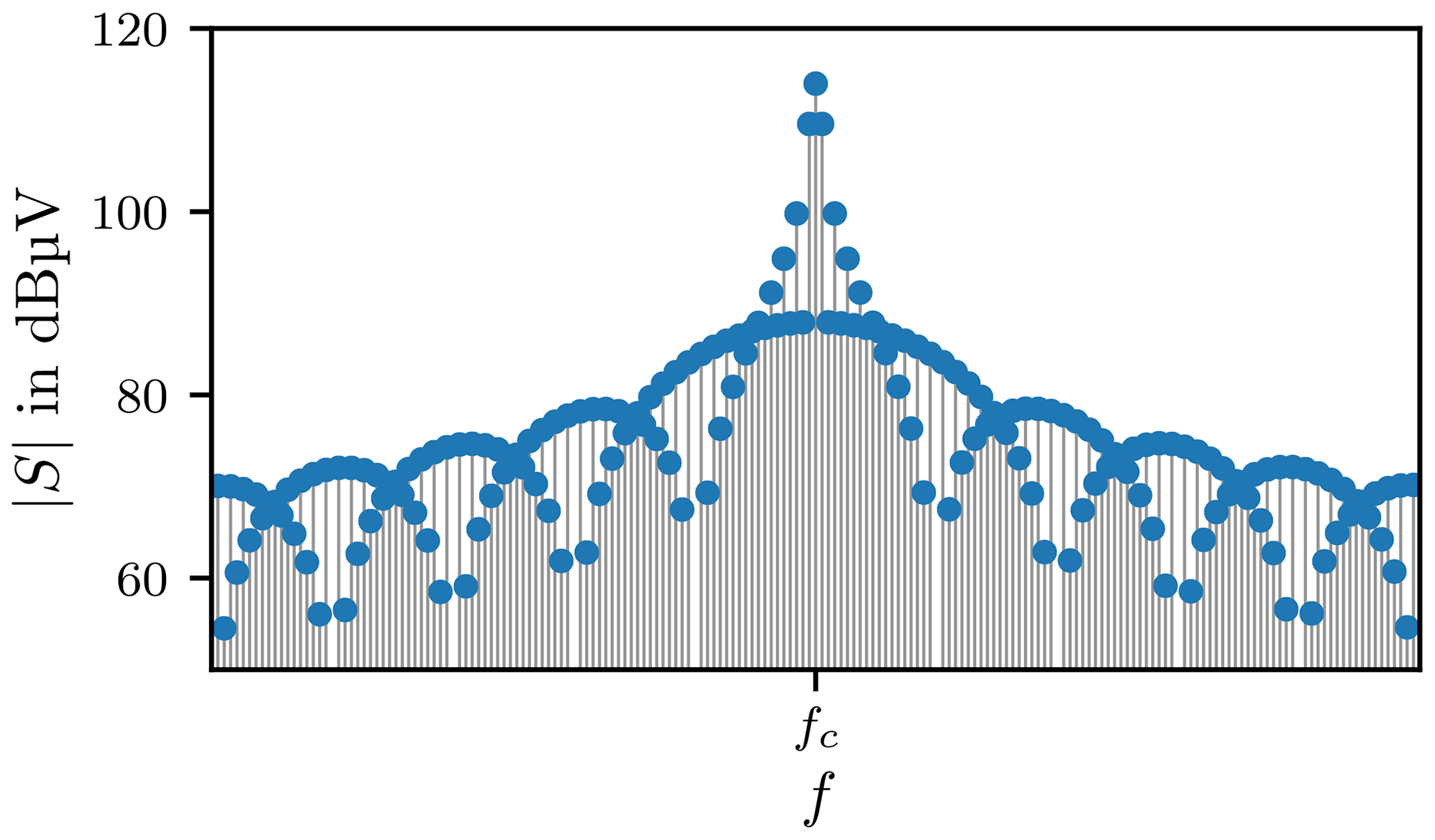
These coefficients determine the spectrum of the idealised pulsed signal with
and is shown in Fig. 4. The rise and fall times are finite in practice which limits the bandwidth (Pozar, 2005).
To generalise the processing of the signals, it is beneficial to decompose the signal into its carrier and envelope parts. In a first step the analytic signal ua(t) must be computed from the real signal u(t) with the Hilbert transform.
The Hilbert transform is defined as
and the inverse transform as
The integral representation of the Hilbert transform in Eq. (17) corresponds to the convolution integral, thus the transform can also be represented as
where ⋆ represents the convolution operation similar to Eq. (17). Using ⋆ the inverse Hilbert transform is
with as the kernel of the Hilbert transformation.
In contrast to the Fourier Transform the Hilbert Transform does not change the domain, u(t), v(t)∈ℝ, see Eqs. (17) and (18). With the usage of Hilbert transform pairs the analytic signal ua(t) becomes
The Fourier transform of the kernel is given by
with the signum function defined as
Expressing the spectrum of ua(t) in terms of the Fourier Transform U(f) of u(t) leads to
In Eqs. (25) and (26) use has been made of the linearity property of the Fourier transform, see Hoffmann (1998), and of Eq. (23).
Evaluating Eq. (26) leads to
The analytic signal ua(t) in its polar form
with the envelope , the complex envelope , the instantaneous phase φ(t) and the carrier frequency f. The complex envelope is given by
the envelope
and the instantaneous phase
The transition from a time continuous signal u(t) to a time discrete signal u[k] is denoted by
with index k∈ℤ and the sample interval Δt.
As noted in Sect. 2 the RC is an oscillating system and can be modelled as a network of RLC circuits. Therefore the different excited modes can be modelled as a sum of exponential functions, see Sects. 6 and 7.
4.1 Measurement setup
Figure 5 shows the measurement setup.
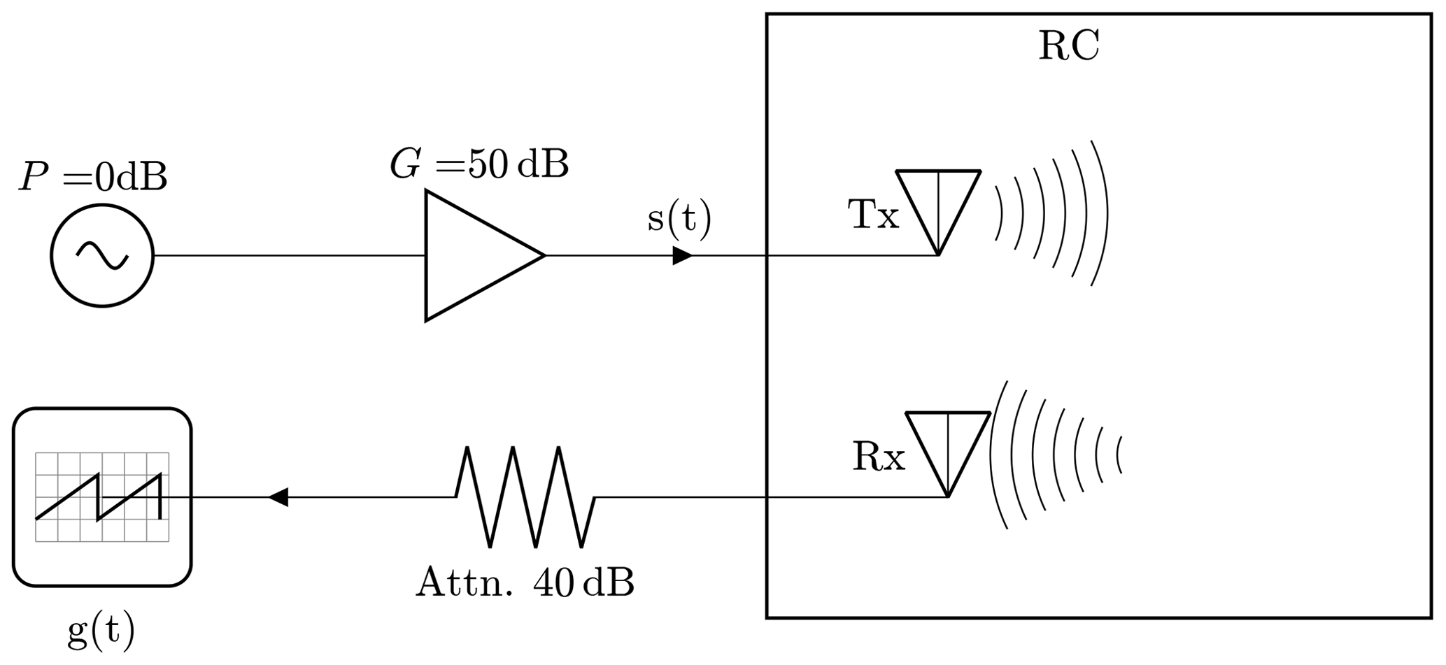
A generator and an amplifier delivers the signal s to excite the RC employing the tx antenna. To record the chamber response g, a real-time oscilloscope is wired to the rx antenna of the same type as the tx antenna.
The carrier frequency fc of the input signal is 400 MHz, with tH=3 µs and tL=7 µs. The power P of the input signal is set to P=50 dBm, which implies A=70.7 V in a 50 Ω system. The mode density is 8.74 modes per MHz, as calculated in Sect. 2. Figure 6 depicts the spectrum of the input signal in the frequency range from 395 to 405 MHz and the resonant frequencies, indicated by the vertical lines in the lower bar.

The input signal excites several modes simultaneously which can lead to high field intensities in the chamber.
4.2 Signal preprocessing
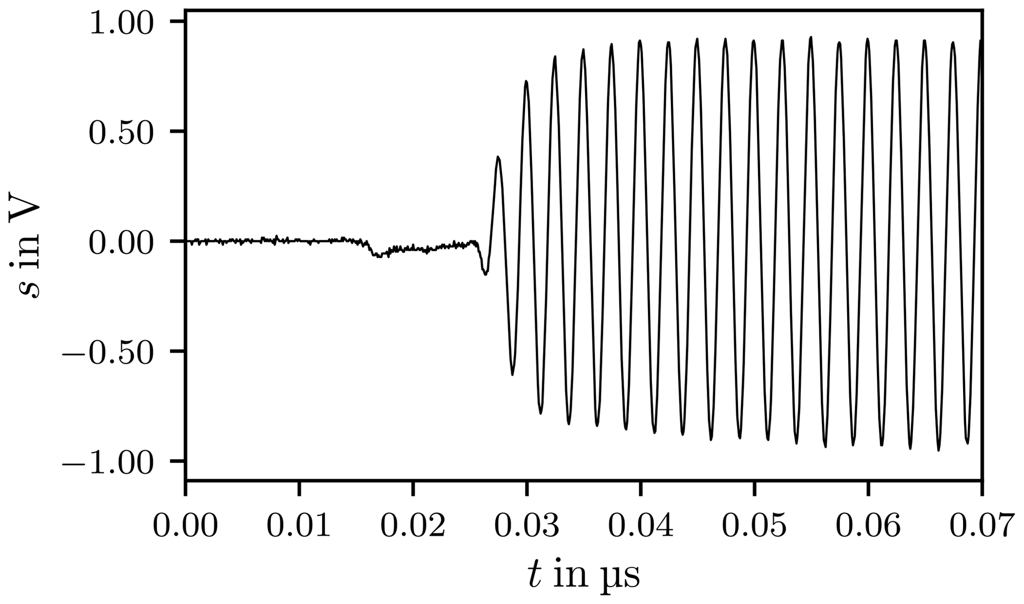
Figure 7 depicts the actual signal applied to excite the chamber when the carrier is switched on and Fig. 8 displays the signal when the carrier is switched off, where the curves clearly reflect the finite rise and fall times. The signal described in Eq. (6) has infinite rise and fall times it is therefore an idealisation of the actual signal.

The discrete Fourier Transform (DFT) of the actual input signal is computed employing the Fast Fourier Transform (FFT) algorithm. Figure 9 shows the spectrum of the signal sampled with the sample frequency fs=25 GHz. At 400 MHz the peak of the carrier frequency is clearly visible. The dashed red box indicates the operational frequency range of the antennas according to the data sheet as their transfer functions are not known. The red arrows mark the harmonic distortions caused by elements with a non-linear transfer function, for instance the amplifier, other intermodulation products are also visible.
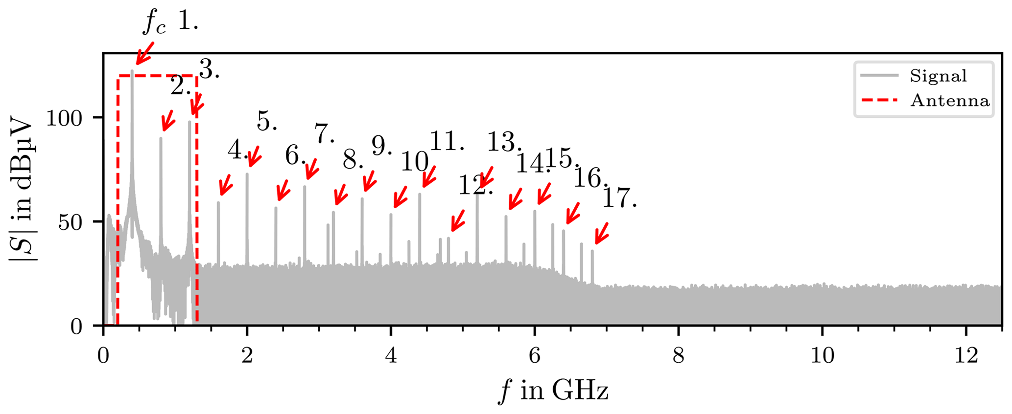
Figure 9Spectrum of the input signal S(f). The red arrows mark the harmonic distortions. The dashed red box shows the frequency range of the antennas.
These frequency components will excite modes in the RC, because of the LTI nature of the system. To filter these unwanted frequency components from the chamber response a 4th-order Butterworth band-pass filter is used, with a bandwidth of 200 MHz.
The spectra of the idealised and of the actual signal are symmetrical with respect to the carrier frequency in displayed frequency range.
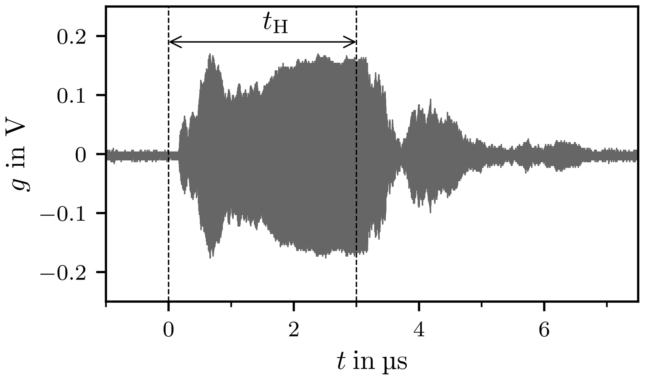
Figure 10 shows the response of the chamber in the time domain, sampled with fs=2.5 GHz, where the dashes lines mark the trigger points when the carrier is switched on and off. After the trigger signal a delay of approximately 140 ns is observed, this signal propagation delay tD is caused by the amplifier, cables and connectors. The propagation delay is frequency dependent because the transfer functions of the amplifier, cables and connectors are frequency dependent.
The spectra of the actual input signal and the chamber response differ which implies that transfer function of the RC is frequency dependent. The peak value at the carrier frequency is decreased by 25 dB corresponding to the insertion loss of the chamber.
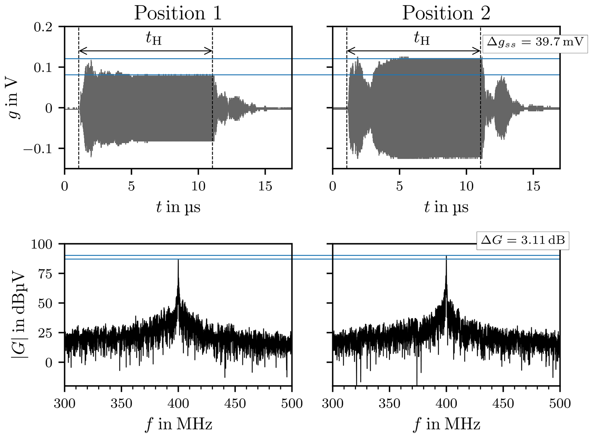
Figure 11 shows two chamber responses and their Fourier transforms for different stirrer positions. In time-domain the responses show different characteristics, such as settling time, overshoot and quasi-steady-state value. In frequency-domain the only observable difference is the derivation of the peak value at the carrier frequency, corresponding to the different quasi-steady-state values, indicated by the blue lines in the figure.
In Fig. 12 the black trace indicates the envelope of the chamber response, it is visible that the envelope is noisy. Figure 13 shows a chamber response for the same stirrer position as Fig. 12, where the acquisition mode is changed from single shot to average mode. In average mode the oscilloscope averages over N=150 successive traces. The envelope appears to be less noisy. This indicates that the envelope is superimposed by a mean-free white noise which does not contain any information.
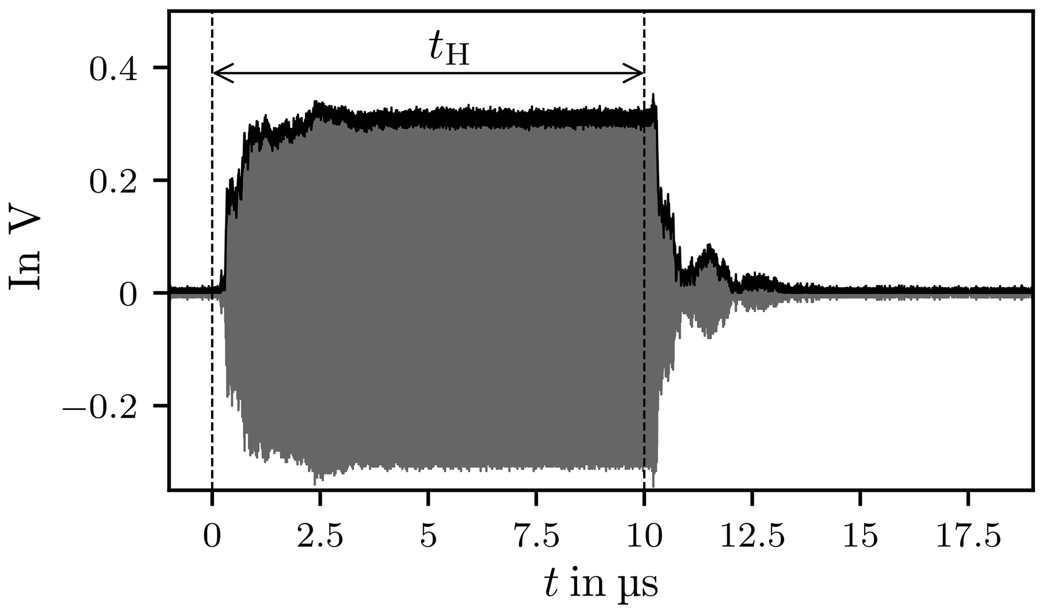

Figure 14 shows the spectra of the single shot and the averaged trace, the spectrum of the averaged signal has a sharper peak at the carrier frequency and the noise floor is significantly reduced and so the signal-to-noise ratio increased. The peak at 800 MHz is the second harmonic of the carrier frequency, generated by the signal generator or the amplifier.
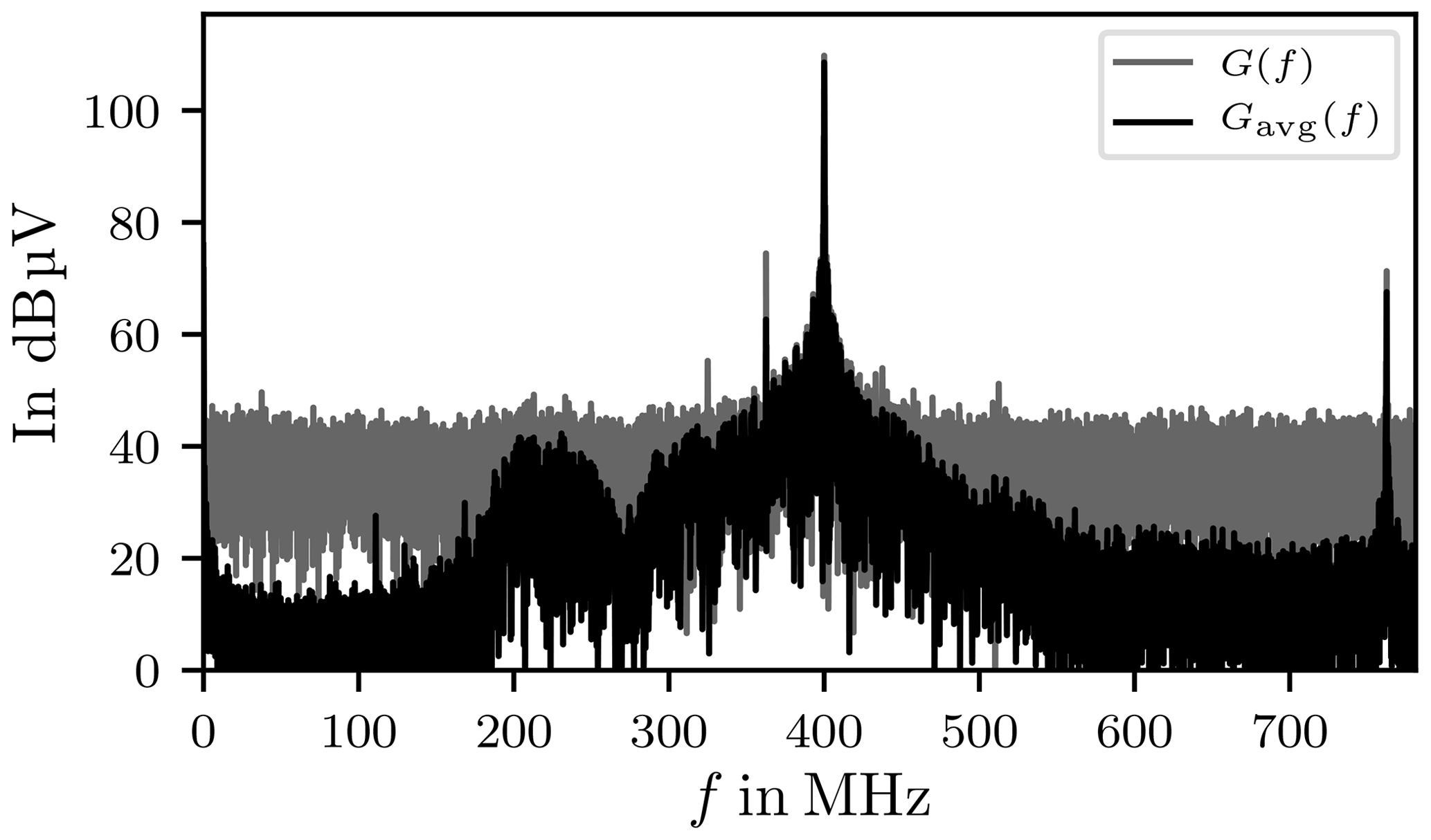
Figure 14Spectra of chamber response, recorded with single shot G(f) and average mode Gavg(f).
Figure 15 shows the spectrum of the filtered chamber response g[k] and its complex envelope , see Eq. (31). The spectra is band-limited and centred around f=0 Hz.
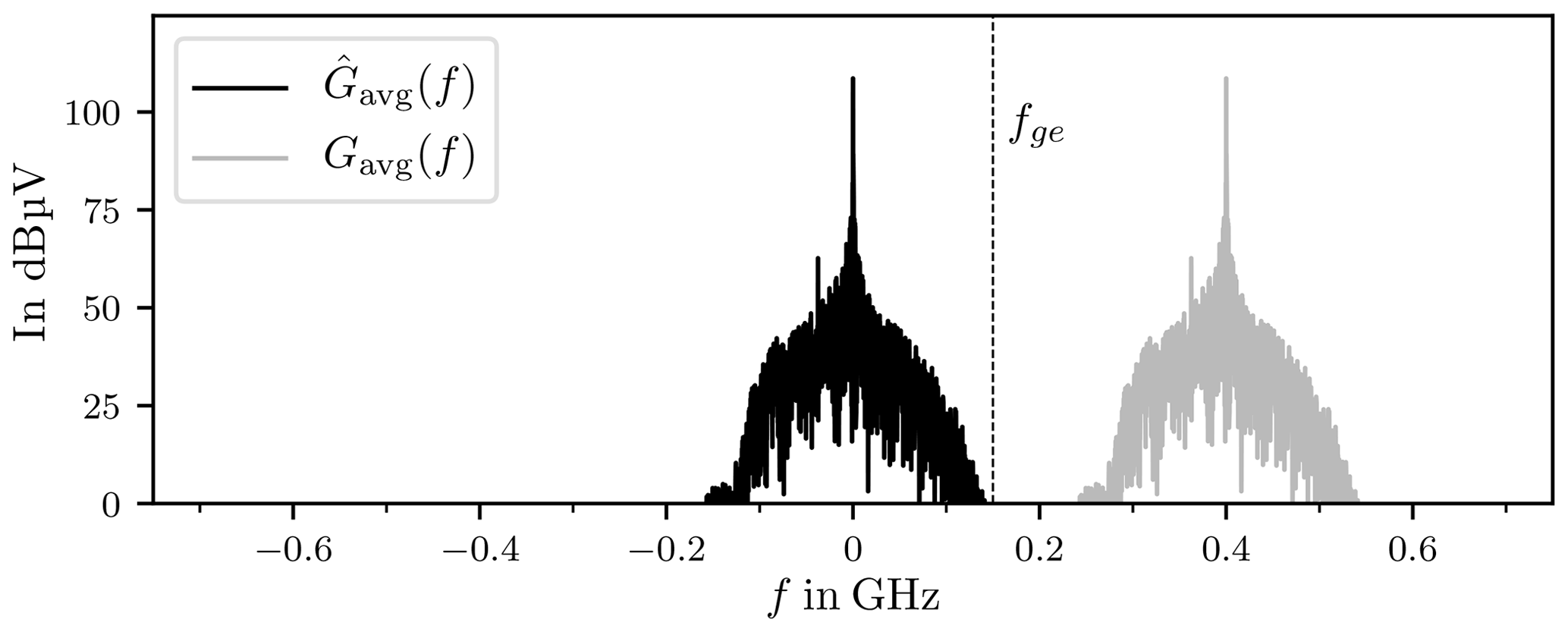
It is now possible to downsample the complex envelope of the chamber response, because the upper frequency limit fge of the complex envelope is much smaller than the upper frequency limit fg of g[k].
The signal g[k] has P samples with k∈Ik and
To downsample g[k] it must first be multiplied with a D-periodic sequence of unit pulses
with the decimation factor D
The downsampled signal consists of every Dth value of g[k]
and the sample interval Δtu
The signal gu[k] consists of samples with and
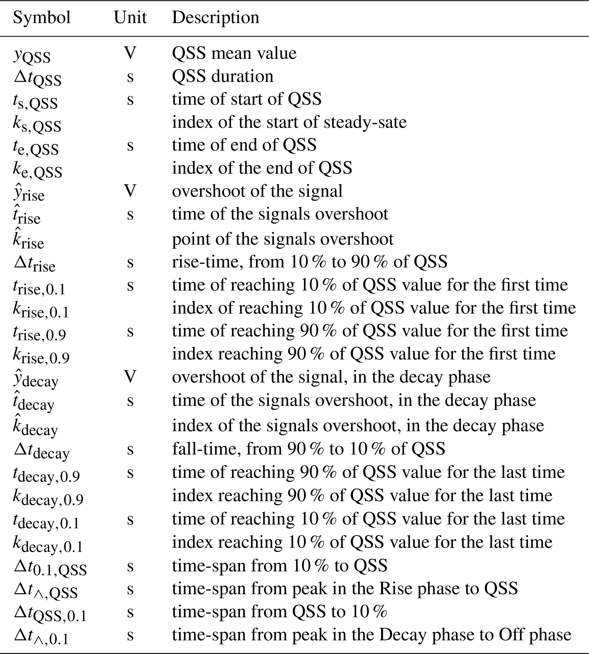
In this section an algorithm is presented that extracts signal properties like rise time and overshoot amplitude. Table A1 lists all properties of interest. This algorithm works on a single chamber response, in contrast to Artz (2017) which needs to process a whole set of measurements first.
The averaged downsampled envelope of the input signal su,avg is designated as the input signal x and the averaged downsampled envelope of the chamber response is defined as the output signal y
5.1 Outline of the algorithm
In order to extract the signal properties of interest the signal is partitioned into four parts
-
rise phase,
-
quasi-steady state (QSS),
-
decay phase,
-
off phase.
First, the limits of the quasi-steady state are identified. Knowledge of the quasi-steady state allows to derive the start and end points of the remaining phases. A sequence of tasks is necessary to determine the start and end point of the quasi-steady state. These steps are
- i.
smoothing of the envelope,
- ii.
clipping,
- iii.
computation time-derivative,
- iv.
deriving threshold for detecting the quasi-steady state,
- v.
identification of start and end points.
With the location of the quasi-steady state the amplitude is estimated. The algorithm concludes with the determination of the requested signal properties from the previously computed results.
5.2 Algorithm
In the following section the single steps for the determination of the quasi-steady state are presented.
5.2.1 Smoothing
Signal smoothing is accomplished by employing a Savitzky-Golay filter, see Savitzky and Golay (1964). In our example we used a window length of 83 and a polynomial degree of 3.
5.2.2 Clipping
The quasi-steady state has to be within the boundary of the trigger time and the switch off time, see Fig. 16, which mark the utmost limits of the QSS. This time-span covers the Rise phase and the QSS. All signal values outside of the interval are neglected. The index of the trigger time, the trigger point kT, and the pulse width tH is known. The start point and the end point of the clipped signal are
In Sect. 4.2 a propagation delay was observed in the chamber response right after the trigger point. This delay is taken into account by shifting the former start and end points (Eq. 44) to
where tD=140 ns. This gives the clipped signal
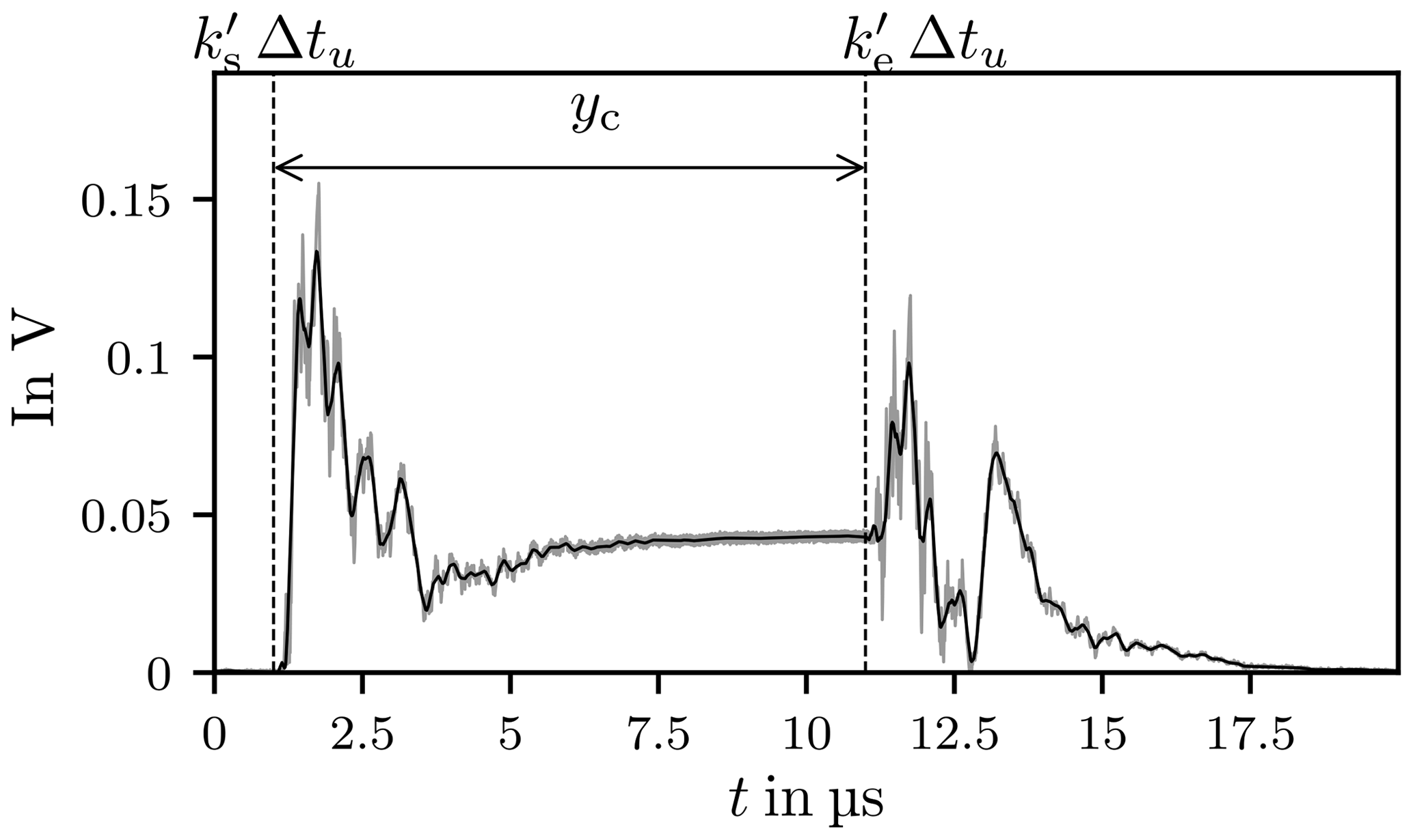
Figure 16The envelope of the chamber response in grey, the smoothed signal y in black and the time-span of the clipped signal yc is indicated by the vertical dashed lines.
5.2.3 Time-derivative
An ideal QSS is defined by a constant amplitude over a certain time period. The derivative for this time period is zero. In practice a deviation around zero is expected and an alteration limit needs to be defined, see Fig. 17.
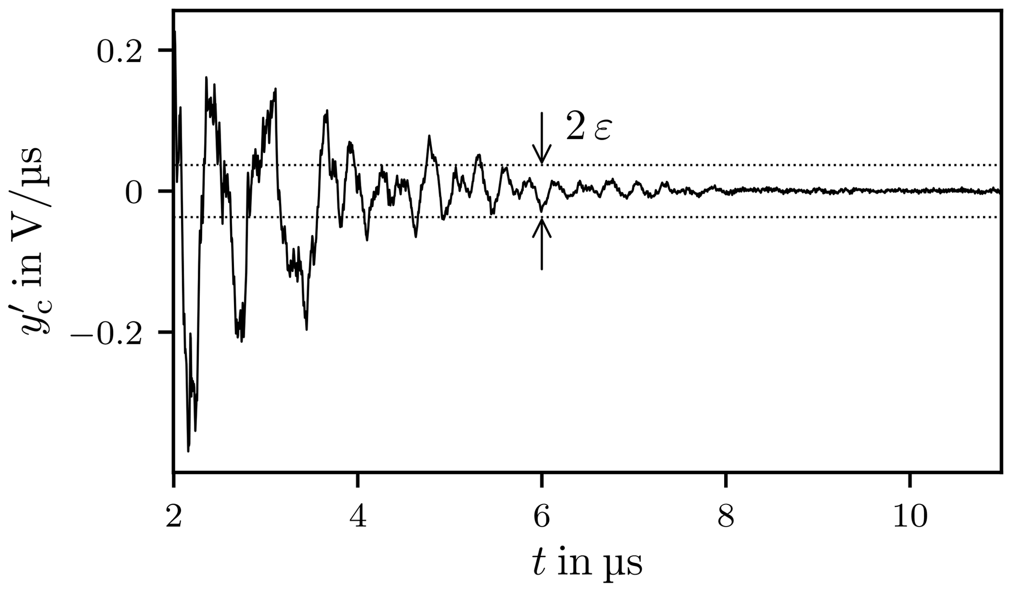
The time-derivative is calculated with a forward-difference quotient
5.2.4 Threshold determination
In order to determine the maximum deviation around zero for the QSS a cumulative histogram is used, see Fig. 18. The ordinate is restricted to the main interval I which is partitioned into N sub-intervals
The boundaries of the sub-intervals , ku,j] are the edges of the bin bj, which is the cardinality of Ij
A threshold for the QSS value is obtained from the lower boundary of the interval . The index of this interval nQSS has to fulfil the condition
where
The threshold is
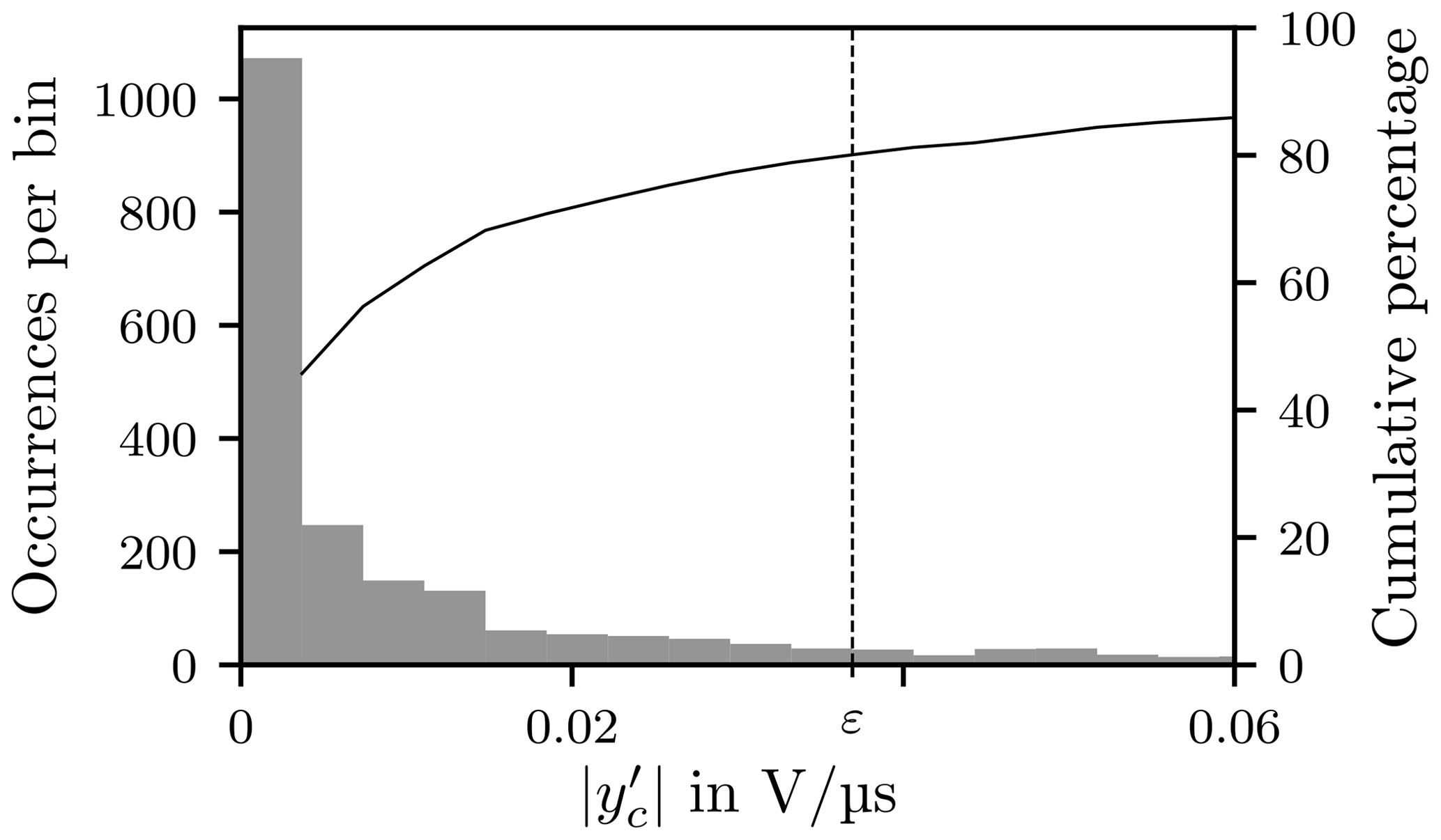
Figure 18Histogram with 100 bins of equal width, the cumulative percentage and the threshold ε. The x-axis is truncated at 0.06 V µs−1 to increase the readability.
5.2.5 Start and End Point of the QSS
In the final step of the algorithm the start and end points of the QSS are determined. The QSS is defined by coherent regions where every value has to be smaller or equal than the threshold. These regions are
with , the window length L and
If multiple regions satisfy the criterion and if these regions contain subsets of the previous regions they are merged into one coherent region. If the distance ΔtG between subsequent but disjoint regions is small enough the gap is neglected. In our case we used a maximum gap size of
with δ=200. The merging process can have one of three possible outcomes. Either no region, one region or multiple disjoint regions are found. When no region is found no QSS exists.
The optimal outcome is that only one coherent segment results from the process. The identification of the QSS is obvious.
If more than one coherent segment have been found, the longest segment is chosen as the actual QSS.
Where y[k] is now divided into five segments
with
and
The QSS mean value is
5.3 Results
The previously determined steady-state value yQSS is now used as a normalisation parameter to simplify comparability between different chamber responses
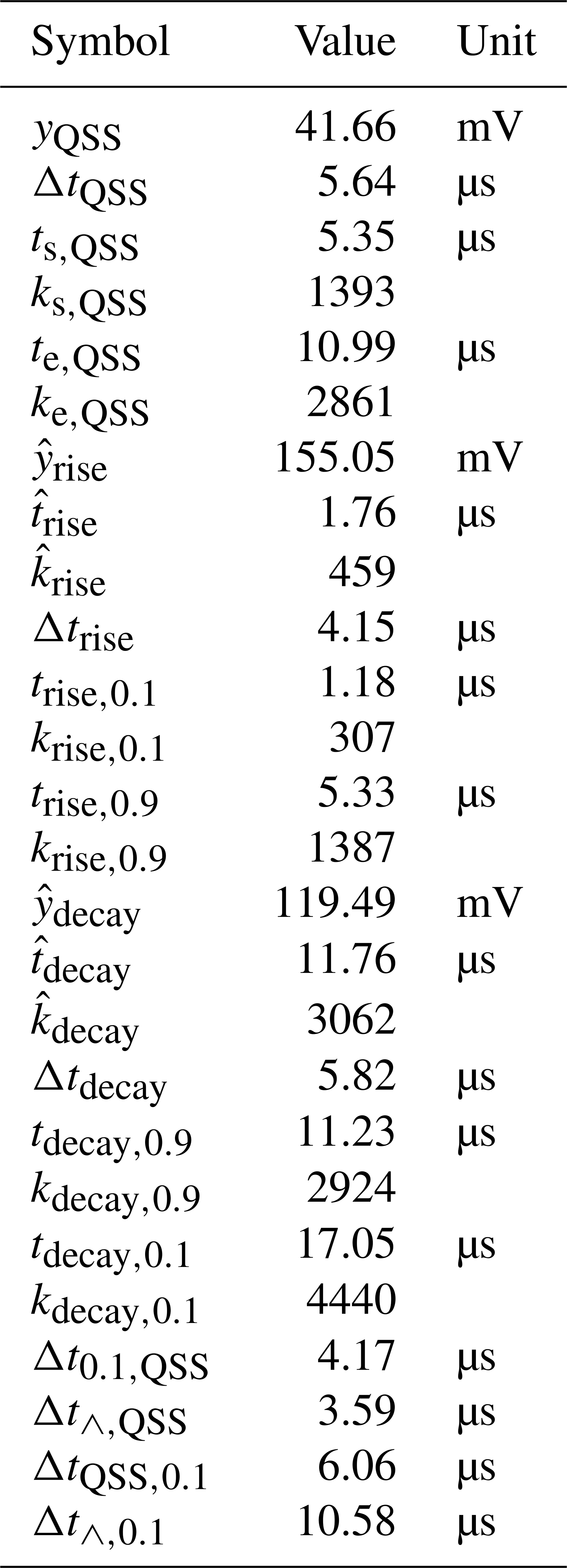
An exemplary result is presented in Fig. 19 consisting of a measured noisy signal y[k] and its noise reduced part. The extracted boundaries for the four signal states are indicated by dashed vertical lines, further properties are listed in Table 1.
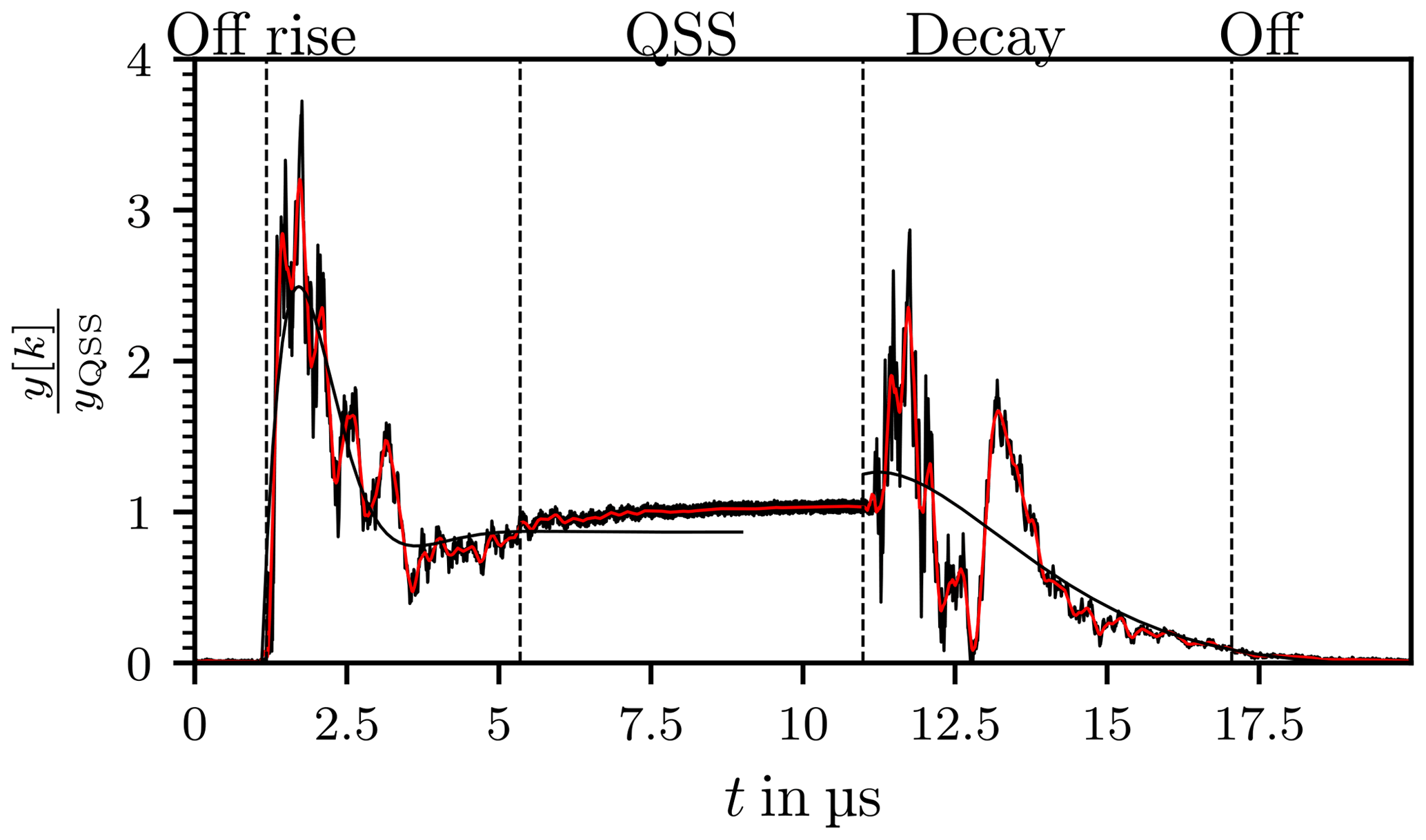
Figure 19The envelope of the chamber response in black, the smoothed signal y in red. The vertical dashed lines indicate the limits of the signal parts. The Rise and the Decay phase are approximated with damped oscillations.
Due to the oscillating nature of the measured signals, the system responses are interpreted as oscillating systems. Based on this assumption it is possible to determine time constants for the rise and fall of each signal. A simple damped harmonic oscillation is
where A, B, C, T and W are unknowns and to is a known shift along the t-axis. The sought-after time constant is then T−1.
Computation of the unknowns in Eq. (58) is accomplished with the help of a Levenberg–Marquardt routine, an iterative trust-region algorithm (Marquardt, 1963). A necessity for convergence are well-posed starting values. Those values are obtained through a reduced model for A and T
described in Appendix A. The starting values for the fitting process are then
The determined time constants for the chamber response depicted in Fig. 19 are for the the Rise and Decay phases
The described algorithm is now applied to a series of measurements of L chamber responses. Measurements were taken over a full stirrer rotation at a stirrer step size of 1∘, this leads to L=360 chamber responses. The measurement setup corresponds to that described in Sect. 4.1.
The distribution of incidences of selected properties are shown in Figs. 20–22. Those properties include the QSS value yQSS, QSS mean value normalised to the pulse width
and the peak value in the Decay phase . The bins are of equal width.
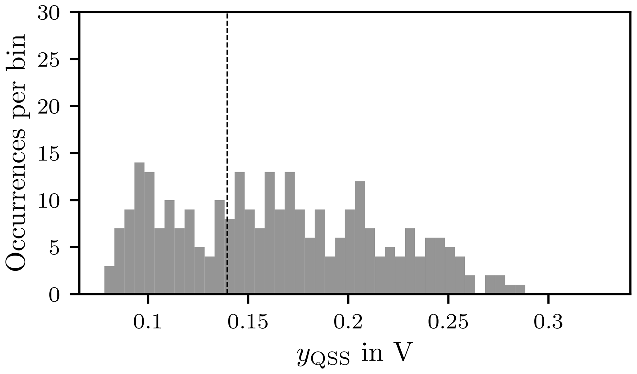
Figure 20Histogram of the QSS mean value yQSS with 50 bins. The dashed line indicates the mean value.
In Table 2 the population mean
and the population standard deviation
as a measure of spread are computed for the three properties.
Table 2Population mean μ and standard deviation σ computed for selected properties.

The standard deviation indicates a wide spread around the mean value of the yQSS. This means that the field strength varies notably over the DUT for a full stirrer rotation.
Figure 21 shows the distribution of incidences of the duration of the quasi steady state in relation to the pulse width, it can be seen that the QSS value is present on average for only 57.1 % of the pulse width (Table 2).
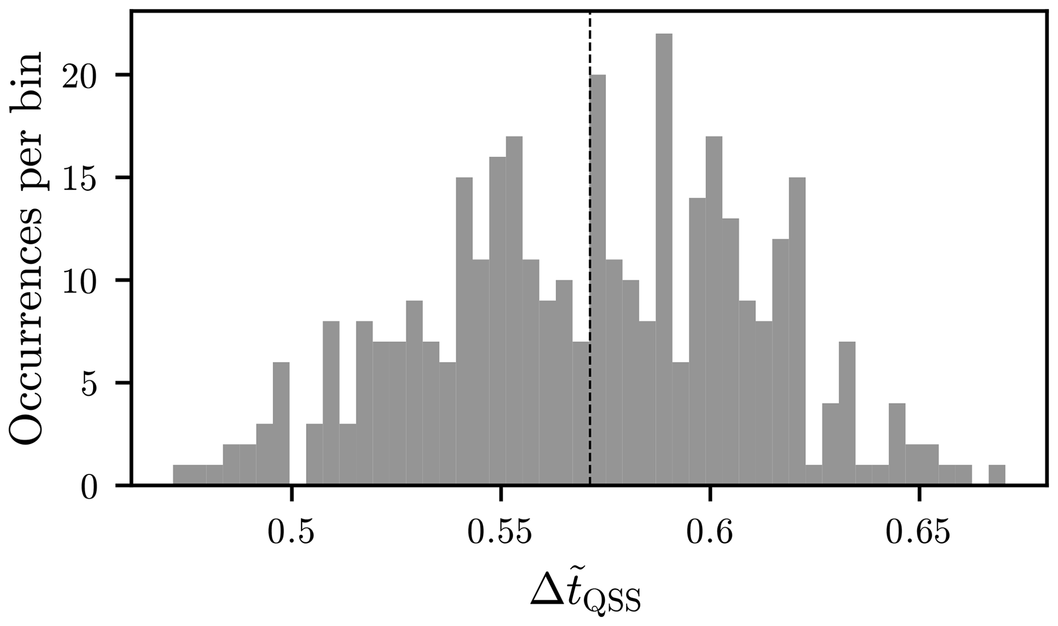
Figure 21Histogram of the QSS mean value normalised to the pulse width tH, with 50 bins. The dashed line indicates the mean value.
The spread of the peak values in the Rise and Decay phase around their mean value is smaller than for the QSS mean value. In the histogram this can be seen by an accumulation of values around the mean value in Fig. 22.
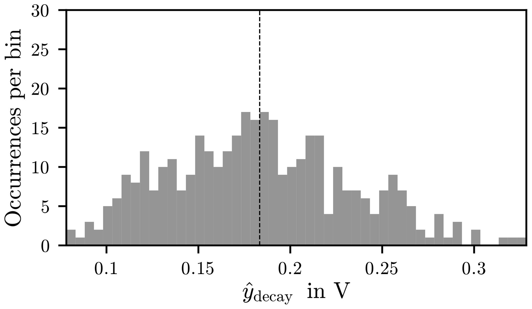
Figure 22Histogram of the peak values in the Decay phase , with 50 bins. The dashed line indicates the mean value.
The relationship between the overshoot and the QSS mean value is shown in Fig. 23. Each QSS mean value yQSS is the reference value to the corresponding overshoot of the data set. A corresponding example is given in Table 1 and the explanation of the symbols is given in Table A1. The overshoot decreases with increasing QSS mean value, this is in agreement with Artz (2017). This indicates that in this case, with the appropriate choice of test parameters, over-testing will not occur.
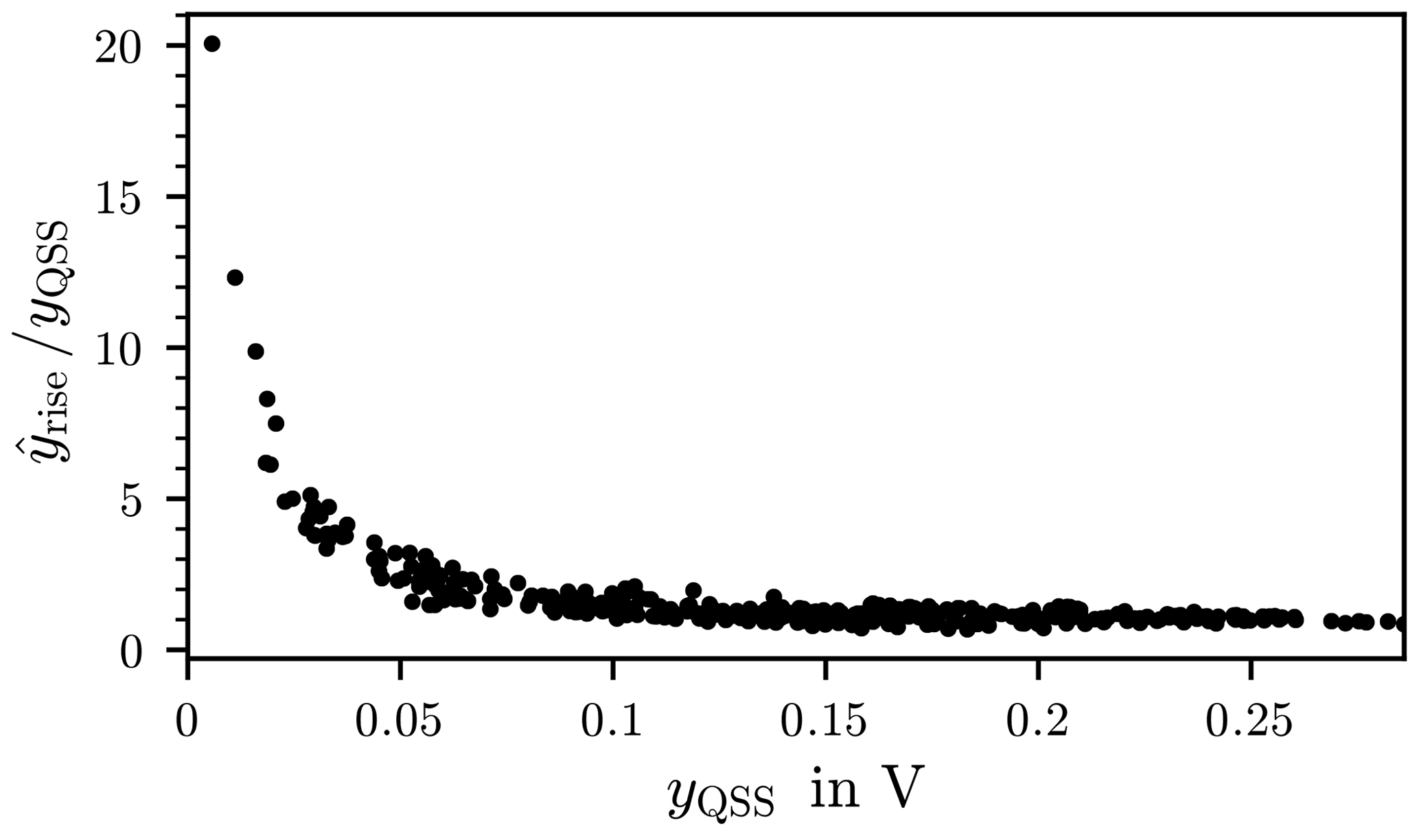
Figure 23Plot of the signals overshoot normalised to the corresponding mean value in the quasi steady-state yQSS over the mean value in the quasi steady-state.
The results of the algorithm are the foundation for further investigations.
With Prony's Method a decomposition of a signal into a sum of weighted complex exponentials can be performed (Marple, 2019; Hauer et al., 1990). From this representation Amplitude, phase shift, attenuation and angular frequency can be determined.
Prony's Method is sensitive to noise (Marple, 2019; Peter, 2013), it is recommended to reduce noise in the input signal before applying the method. Noise reduction is achieved by the signal pre-processing described in Sect. 4.2.
6.1 Description of the method
The signal y[k] is approximated with
where M≥2p and
is an amplitude, Ωn a phase shift, αn a damping factor and fn is a frequency.
The unknown factors appear linear as pre-factors hn and non-linear as arguments of an exponential function zn. These unknown parameters are determined in two steps. First the exponents are determined and then the coefficients.
The core of Prony's method is the assumption that the sum of the exponential functions satisfies a pth order difference equation
(Hamming, 1987). The characteristic polynomial of this difference equation is
where am∈ℝ. The z of Eq. (62) are the zeros of Eq. (66), which are either real or conjugate complex. To determine these zeros, the coefficients a0, …, ap must be known. If a0=1, a linear system for the unknowns a1, …, ap is obtained from Eq. (65) as
With the exponents z determined from Eqs. (66) and (67), the coefficients h1, …, hp can be calculated from the data. Re-writing Eq. (62) in matrix notation gives
From the roots zn, n=1, …, p the searched for arguments of the exponential functions are
The linear coefficients hn give the parameters
The approximated data set is written as
In Eqs. (67) and (68) the matrices are square and can get very large for big sets of data. But in practice the number of data points exceeds the number of unknowns in the exponential model (Eq. 62). This will lead to non-square matrices where the number of data points exceeds the number of unknowns. Various methods are available to solve these over-determined linear systems, for example least squares (Marple, 2019; Peter, 2013). In the present case the least squares approach is used. The method was tested on the transient and decay behaviour of the curve in Fig. 19. The necessary parameters such as the beginning and end of the corresponding phases were taken from Table 1. The data set for the transient oscillation comprises M=1133 data points and p=380 summands were chosen. The actual and approximate course is shown in Fig. 24. There is a very good agreement up to t=3 µs, after that the curves deviate noticeably. The approximation can be improved by increasing the summands in Eq. (62).
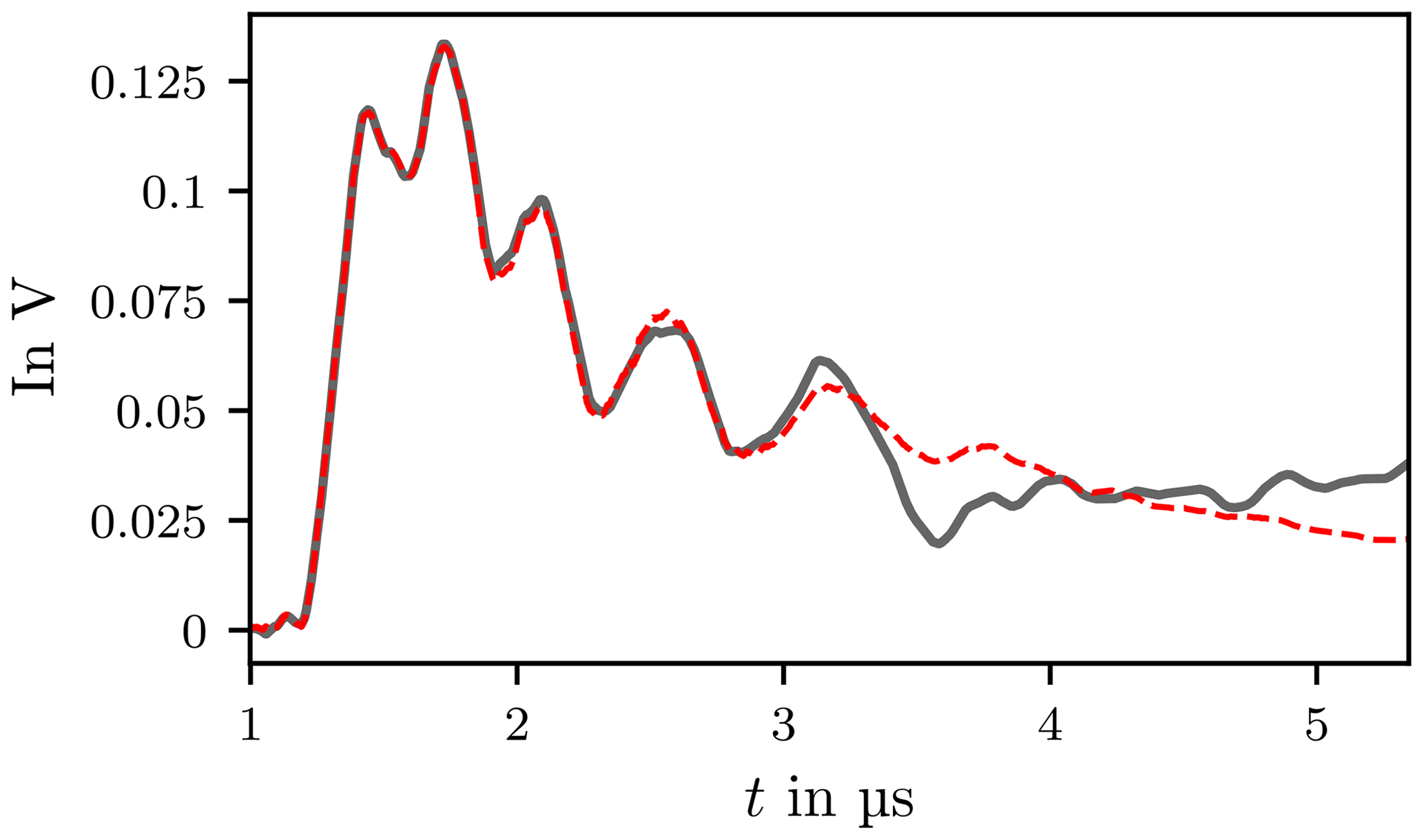
Figure 24Rise phase of signal y[k] and Prony interpolation . The black line is the rise phase of signal y[k] and the dashed red line is the Prony interpolation .
The data set for the Decay phase includes M=1579 data points and p=450 parameters were used. The approximation and the actual course agree well up to about 13 µs (Fig. 25).
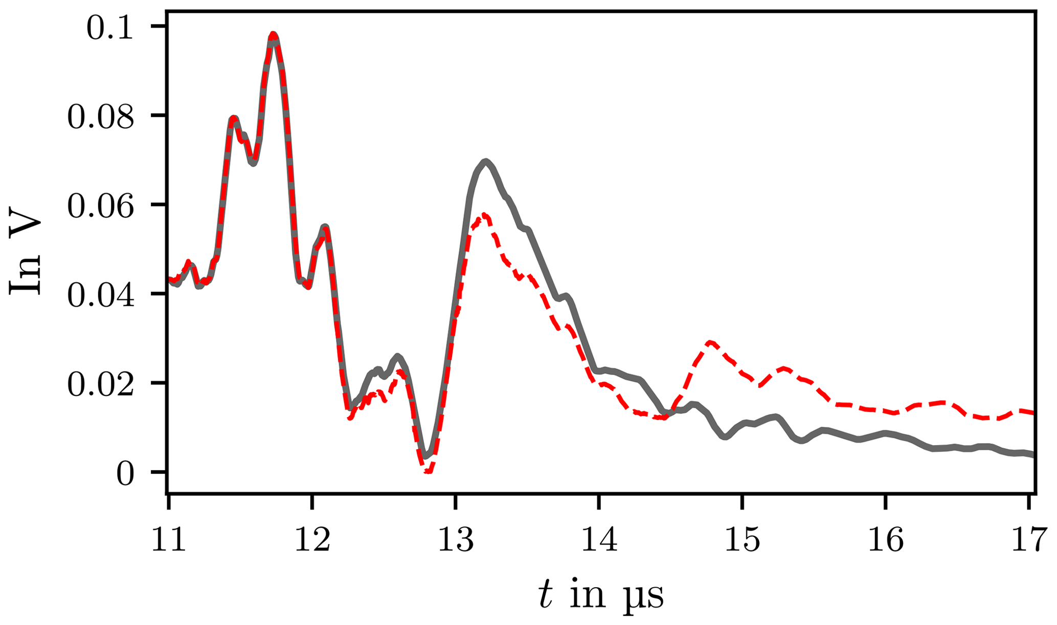
Figure 25Decay phase of signal y[k] and Prony interpolation . The black line is the decay phase of signal y[k] and the dashed red line is the Prony interpolation .
Figure 26 shows the poles according to Eq. (66). A strong spread of the angular frequency is visible. However, since it is a smoothed and band-limited signal, some of the poles found lie outside the permissible frequency band. This means that the curves interpolated with the Prony method contain frequency components which are not physical. Band-limiting leads to a deterioration of the interpolation.
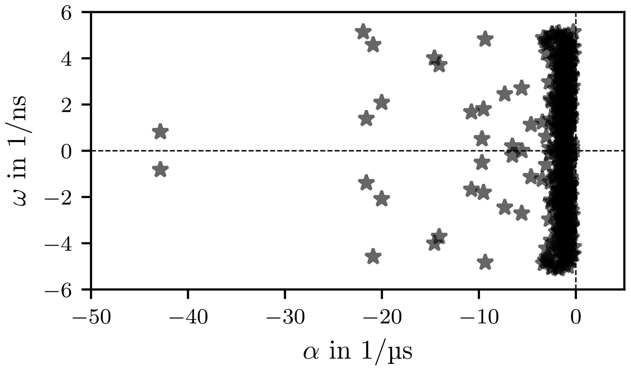
An alternative interpolation method is the TD-VF where pole locations within a given frequency band are selected.
Prony's method represents the measured chamber response as a sum of exponentials. This sum is the result of a convolution of a transfer-function and an excitation. Purely employing Prony's method makes it difficult to extract information about underlying characteristics of the signal transfer. An alternative method is Time-Domain Vector-Fit (TD-VF), which is based on the Vector-Fit (VF) algorithm (Gustavsen and Semlyen, 1999; Triverio, 2019).
Vector-Fit offers the possibility to approximate a transfer-function to a measured response. In the following sub-sections are VF and TD-VF briefly summarised. Afterwards an application to measured data is presented.
7.1 Fundamental vector-fit
The VF method approximates a rational function to frequency domain data using an iterative least squares technique. The transfer-function in frequency domain is
with Y(s) the result, H(s) the transfer function, X(s) the excitation and s a complex frequency parameter. The VF approximation of H(s) is
where d is a constant, Rn the nth residue to the pole pn and N the number of real poles. The iterative least squares approximation is based on an initial set of poles, which are distributed either linearly or logarithmicaly over the investigated frequency range (Grivet-Talocia and Gustavsen, 2016). The main idea in VF is to weigh the input with a function σ
and enforce the product σ(s)H(s) to match the left-hand-side, with
and
Letting X(s) to be unity, then the unknowns d, Kn and form a linear least-squares problem for every data point Y(si)
i=1, 2, …, Mf, where Mf represents the number of frequency samples. When the least-squares problem has reached a solution, then the new poles for H(s) are the zeros of σ(s)
With the relocated poles the original problem (Eq. 75) is an over-determined linear system in the unknown residues Rn.
7.2 TD-VF
Similar to the VF in frequency domain the TD-VF solves a linearized least-squares problem in time domain based on a known excitation x(t) and measured response y(t) (Grivet-Talocia, 2004). Applying an inverse Laplace transformation on Eq. (74) leads to
The approximated time domain transfer-function is
with δ(t) the Dirac-function and 1(t) the unit step function. In order to determine the transfer function h(t) an estimate for initial poles has to be given first. Afterwards, a least-squares solution for the unknowns similar to Eq. (79) allows to determine relocated poles. Equation (79) in time domain is
The computationally demanding task of evaluating the convolution integrals simplifies with the usage of a recursive convolution algorithm (Semlyen and Dabuleanu, 1975). With the previously determined poles equation (Eq. 82) allows for the determination of the residues Rn in the least-squares sense.
In the case of conjugate complex poles Eq. (83) becomes
with Nr the number of real poles, Nc the number of complex poles, pr,n are real poles and pc,n are complex poles. In Eq. (85) the complex poles and residues appear in complex conjugate pairs, the total number of complex poles and likewise the total number of residues is 2Nc.
If the deviation between approximated response and original response y(t) is smaller than a previously determined threshold the iteration stops. The deviation is evaluated in terms of a two-norm
which is called root mean square (RMS). M is the number of time samples. The vectors y and denote function values for each time step. A normalised error measure is
7.3 Application
The TD-VF is applied to two measurements for two different but fixed stirrer positions and a fixed antenna position within the chamber. Before TD-VF is used a low-pass filter is applied to reduce noise and distortions, the procedure is described in Sect. 4.2.
A common difficulty is the prior knowledge of the number of required poles. So far there is no general procedure available that can solve this problem, apart from iterative solutions. It is possible to locate regions in frequency domain within which poles ought to occur, these regions are in between two local minima. This method is only suitable for frequency responses (Heindl et al., 2009).
The envelope of the excitation signal is depicted in Fig. 27. All following investigations relate to the envelope of the input signal. The reconstructed transfer-function (Eq. 85) is actually the transfer-function of the envelope of the measured response.

In order to determine the transfer-function from Eq. (84) and afterwards from Eq. (82) the following abbreviations are used
The linear system (Eq. 84) is of dimension where one row corresponds to a time step tk
Here Kr,n are real residues according to Eq. (84). Kc,n and denote complex residues
The pole relocation process reduces to an eigenvalue problem (Gustavsen and Semlyen, 1999). The numerically determined eigenvalues have to fulfill the following requirements:
-
The poles have to be stable, which means that the real part has to be negative. If a pole has a positive real part the stability condition
shifts the pole to the left of the imaginary axis.
-
Poles outside of the frequency range (Eq. 99) are not valid poles and are discarded.
-
Each pole has to fulfill
Equation (97) makes use of Eq. (75), where a linearization of the integral leads to a simplified evaluation in the complex s-plane. The problem simplifies further, when a linearized circle with small radius around pn is used as integration domain. This test has been carried out in the AAA-Fit algorithm to detect and discard spurious poles (Nakatsukasa et al., 2018). Grivet-Talocia and Bandinu (2006) investigate further validity conditions also for data that includes noise.
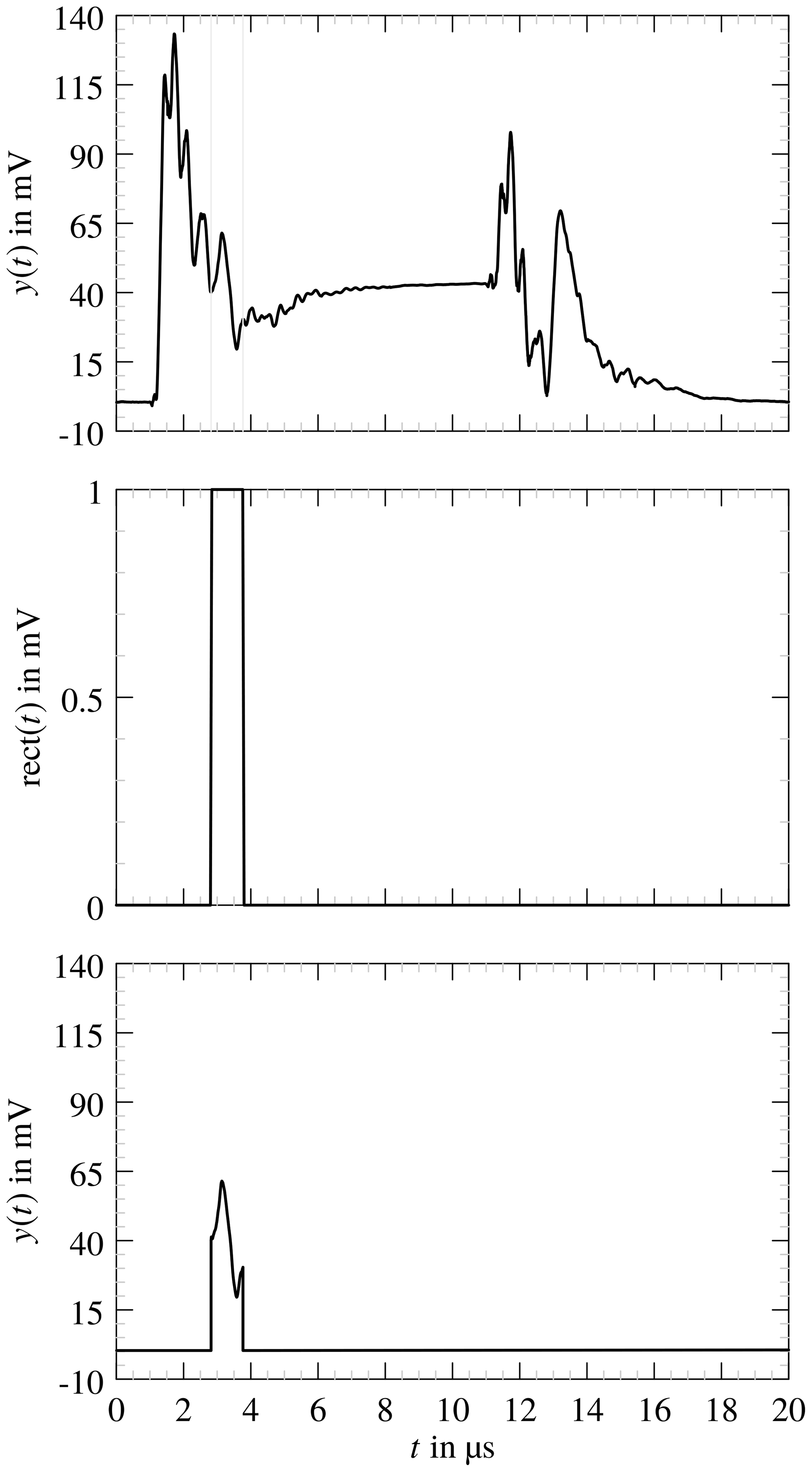
Figure 28Selection of a curve segment and resulting segment that is approximated with TD-VF.
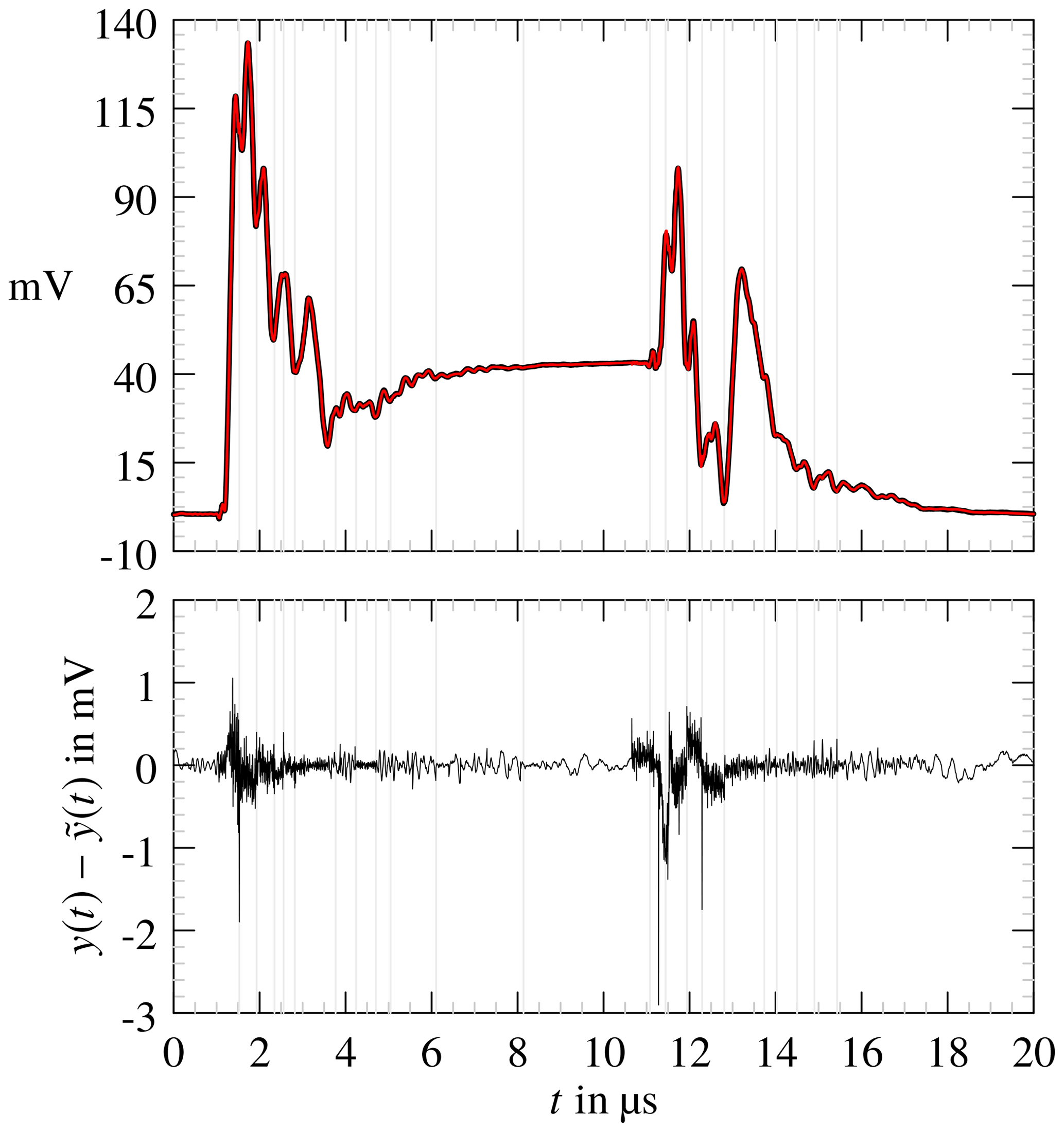
Figure 29Approximated function in red and measured response y(t) in black. Below is the absolute error.
Both data sets consist of M=5000 sample points, with Δt=4 ns. A direct fit of the whole data set did not lead to an acceptable result and should be avoided. It is more convenient to partition the data and fit consecutive parts. An algorithm has been developed that locates minima in the data, which are used as partition boundaries. The overall error is reduced when the approximation is based on a delayed transfer-function (Charest et al., 2010). In Eq. (82) h(t) becomes
where each hi(t−τi) corresponds to Eq. (85). Ns is the number of segments bounded by [τi, τi+1], i=1, 2, …, Ns.
In Fig. 28 is the segment selection process shown. A specific segment is chosen by multiplying the data set with a rectangle, the resulting curve segment is fitted with TD-VF. The start poles are chosen between
where τi+1 and τi are the boundaries for the segment. Since the curve segment is the product of the original data and a rectangle function, a near infinite frequency width would be contained in this signal section. Frequencies that exceed the band limit, which is fixed due to the signal preprocessing (Sect. 4.2), are excluded and the fitting procedure is repeated until a good curve approximation is obtained or until the iteration limit is reached. An approximation is shown in Fig. 29 together with the deviation of the smoothed data set. The RMS is 0.138 mV with Nr=179 and Nc=560 poles. A second example is depicted in Fig. 30 with an RMS of 0.163 mV.
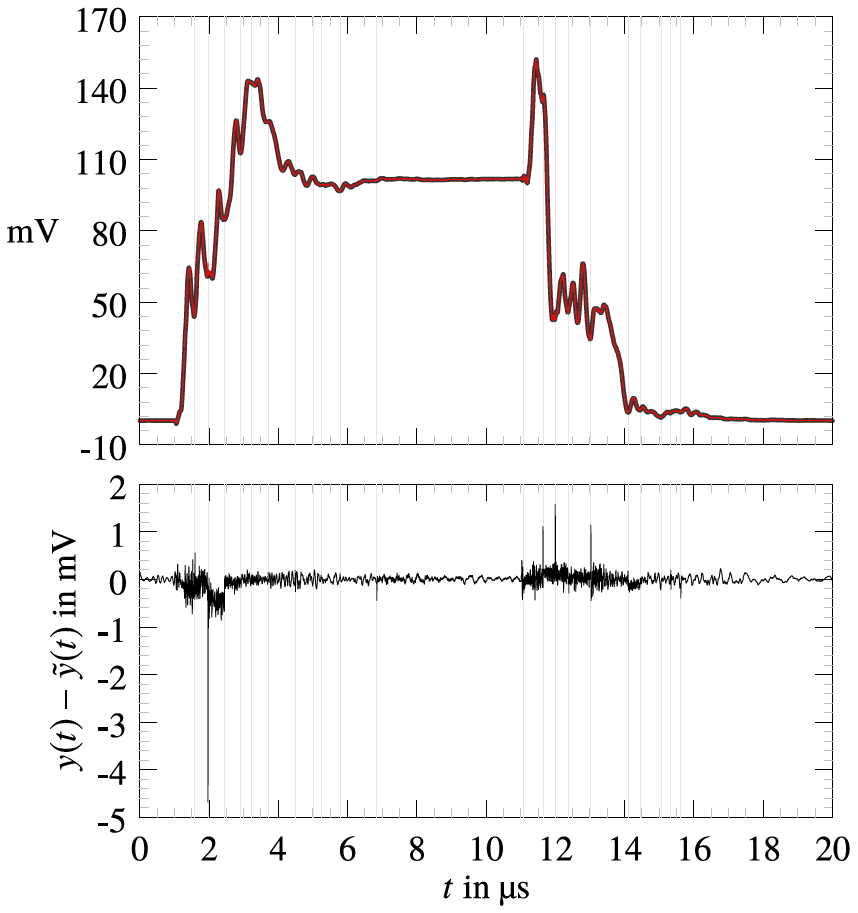
Both approximations fit well to the original curve. A majority of the deviations appear at segment boundaries. Charest et al. (2010) make use of a wavelet decomposition for the response signal, which allows for an algorithmic search for ideal segmentation points. This could not be applied yet and is left for future work.
7.4 Outlook
The TD-VF has been applied on a single measured signal. The signal belongs to a fixed position within the RC-chamber where the stirrer is at rest. The reconstructed signal is based on a transfer-function which is defined through residues and poles according to Eqs. (98) and (85). This transfer-function is not the transfer-function of the RC-chamber rather of the whole system consisting of cables, antennas and the chamber. Knowledge of the transfer-functions of the sub-systems – cables and antennas – give a more detailed description of the chamber, like its eigenmodes.
A multi-resolution in frequency and time gives the possibility to computationally partition the response signals. An automated TD-VF evaluation of signals, each measured at a fixed but different stirrer position, could then construct the transfer-functions systematically.
A system theoretical approach has been presented to explain the transient behaviour of a reverberation chamber excited with a pulsed signal. A spectral analysis on a pulsed signal and on the chamber response has been employed.
The spectrum of the chamber response shows that resonant frequencies in the neighbourhood of the carrier frequency are excited. Chamber responses of different stirrer positions provide nearly identical spectra. Differences between the chamber responses are more visible in the time domain.
An algorithm for the extraction of defined parameters was developed. Distinction of the individual responses is automatically possible on the basis of these parameters. The parameters include, for example, the duration and amplitude of the steady state as well as the time constants for the rise and decay. The results of the algorithm constitute the basis for further investigations, in particular the identification of the steady state is essential.
For further analysis of the chamber the data were approximated by a continuous function. This approximation is based on a superposition of damped oscillations for which the Prony interpolation method was used. The practical implementation is realised by a piecewise approximation of the data whose segmentation requires the knowledge of the steady state.
A similar approach allows to construct the transfer function of the overall RC system from the measurements with known excitation. This method is called Time-Domain Vector-Fit. The transfer function also represents an oscillating system. Similar to the Prony Method, the data set is segmented and approximated piecewise.
However, the approximations are based on linear time-invariant systems, i.e. the stirrer position must be kept constant for a measurement. Further investigations include the simulation of the chamber behaviour based on the approximated transfer functions as a function of the stirrer position. The transfer function of the chamber can be improved by knowing the transfer functions of the individual system components such as antennas, cables and connectors.
Furthermore, a comparison between the two interpolation methods is particularly useful with regard to the parameters obtained, such as the pole points.
To estimate the time constants for the Rise and the Decay phase from a damped oscillation (Eq. 58) start values for the unknown parameters have to be determined first. This is accomplished if a reduced model of a simple exponential process (Eq. 59) is used
One of the searched for quantities still appears in the argument of the exponential function, which would again require a start value for . This can be avoided if Eq. (A1) is rewritten as an integral equation. As a consequence appears the former nonlinear quantity as a linear unknown and the application of classic least-squares is possible (Jacquelin, 2014). Integration of Eq. (A1) with regard to t leads to
The exponential term is expressed with Eq. (A1) and the integral equation
is established, where
and t0 is the starting time value. The sum of the squared error for each time step is
Deriving Eq. (A7) with regard to and results in
which is rewritten as
with
The quantity is discarded in favor of a second minimization based on the determined value of . Simple least squares for and on the basis of Eq. (A1) leads to the desired first order approximation.
All data presented in this article are available from the corresponding author upon request.
FO implemented the TD-VF and the computation of the time-constants. KP conducted the measurements and implemented the Prony Method. FO and KP prepared the manuscript.
The authors declare that they have no conflict of interest.
This article is part of the special issue “Kleinheubacher Berichte 2019”. It is a result of the Kleinheubacher Berichte 2019, Miltenberg, Germany, 23–25 September 2019.
This open-access publication was funded
by the Technische Universität Dresden (TUD).
This paper was edited by Frank Gronwald and reviewed by two anonymous referees.
Amador, E., Lemoine, C., Besnier, P., and Laisné, A.: Studying the pulse regime in a reverberation chamber with a model based on image theory, in: IEEE International Symposium on EMC 2010, Fort Lauderdale, USA, 520–525, https://doi.org/10.1109/ISEMC.2010.5711330, 2010. a
Artz, T.: Transiente Einschwingvorgänge in Modenverwirbelungskammern bei Prüfungen mit gepulsten Sinussignalen, PhD thesis, Universität Duisburg-Essen, available at: https://duepublico2.uni-due.de/receive/duepublico_mods_00044830 (last access: 2 February 2020), 2017. a, b, c, d
Artz, T. and Hirsch, H.: Using the system linearity of reverberation chambers to derive an equivalent baseband model in time-domain to predict the chamber response to an input signal, in: 2014 International Symposium on Electromagnetic Compatibility, 1–4 September 2014, Gothenburg, Sweden, 307–312, https://doi.org/10.1109/EMCEurope.2014.6930922, 2014. a, b
Bernard Demoulin, P. B.: Electromagnetic Reverberation Chambers, Wiley-ISTE, Hoboken, NJ, USA, 2011. a
Charest, A., Nakhla, M. S., Achar, R., Saraswat, D., Soveiko, N., and Erdin, I.: Time Domain Delay Extraction-Based Macromodeling Algorithm for Long-Delay Networks, IEEE T. Adv. Packag., 33, 219–235, https://doi.org/10.1109/TADVP.2009.2029560, 2010. a, b
Deutsche Kommission Elektrotechnik Elektronik Informationstechnik im DIN und VDE: Elektromagnetische Verträglichkeit (EMV) – Teil 4–21: Prüf- und Messverfahren – Verfahren für die Prüfung in der Modenverwirbelungskammer, Standard DIN VDE 61000-4-21, Verband der Elektrotechnik Elektronik Informationstechnik e.V., Berlin, 2011. a
Grivet-Talocia, S.: The Time-Domain Vector Fitting Algorithm for Linear Macromodeling, AEU – Int. J. Elect. Commun., 58, 293–295, https://doi.org/10.1078/1434-8411-54100245, 2004. a, b
Grivet-Talocia, S. and Bandinu, M.: Improving the convergence of vector fitting for equivalent circuit extraction from noisy frequency responses, IEEE Transactions on Electromagnetic Compatibility, 48, 104–120, https://doi.org/10.1109/TEMC.2006.870814, 2006. a
Grivet-Talocia, S. and Gustavsen, B.: Passive macromodeling: theory and applications, Wiley series in microwave and optical engineering, 1st Edn., John Wiley & Sons, Hoboken, New Jersey, 2016. a
Gustavsen, B. and Semlyen, A.: Rational approximation of frequency domain responses by vector fitting, IEEE T. Power Deliv., 14, 1052–1061, https://doi.org/10.1109/61.772353, 1999. a, b
Hamming, R.: Numerical methods for scientists and engineers, 2nd Edn., Dover Publications, Inc., New York, 1987. a
Hauer, J. F., Demeure, C. J., and Scharf, L. L.: Initial results in Prony analysis of power system response signals, IEEE T. Power Syst., 5, 80–89, https://doi.org/10.1109/59.49090, 1990. a
Heindl, M., Tenbohlen, S., Kraetge, A., Krüger, M., and Velásquez, J.: Algorithmic determination of pole-zero representations of power transformers’ transfer functions for interpretation of FRA data, in: 16th Int. Symp. on High Voltage Engineering, Johannesburg, 2009. a
Hill, D. A.: Electromagnetic fields in cavities: deterministic and statistical theories, John Wiley & Sons, Inc, Hoboken, NJ, 2009. a
Hoffmann, R.: Signalanalyse und -erkennung, Springer, Berlin, Heidelberg, 1998. a, b
Jacquelin, J.: Regressions et Equations Integrales, available at: https://www.scribd.com/doc/14674814/Regressions-et-equations-integrales (last access: 26 February 2020), 2014. a
Krauthäuser, H.: Grundlagen und Anwendungen von Modenverwirbelungskammern, in: no. 17 in Res Electricae Magdeburgenses, 1st Edn., edited by: Nitsch, J. and Styczynski, Z. A., Otto von Guericke Universität Magdeburg, Universitätsbibliothek, Magdeburg, 2007. a, b
Krauthäuser, H. G. and Nitsch, J.: Transient Fields in Mode-Stirred Chambers, in: XXVIIth General Assembly of the International Union of Radio Science, 17–24 August 2002, Maastricht, the Netherlands, URSI 2002, 2002. a
Liu, B., Chang, D., and Ma, M.: Eigenmodes and the Composite Quality Factor of a Reverberating Chamber, NBS Technical Note, National Bureau of Standards, availabler at: https://nvlpubs.nist.gov/nistpubs/Legacy/TN/nbstechnicalnote1066.pdf (last access: 3 June 2020), 1983. a
Manicke, A. and Krauthäuser, H. G.: Pulse excitations of reverberation chambers simulations with an approach using time domain plane waves, in: International Symposium on Electromagnetic Compatibility – EMC EUROPE, 17–21 September 2012, Rome, Italy, 1–6, https://doi.org/10.1109/EMCEurope.2012.6396828, 2012. a
Marple, S.: Digital Spectral Analysis: Second Edition, in: Dover Books on Electrical Engineering, Dover Publications, Dover, 2019. a, b, c
Marquardt, D. W.: An Algorithm for Least-Squares Estimation of Nonlinear Parameters, SIAM J. Appl. Math., 11, 431–441, https://doi.org/10.1137/0111030, 1963. a
Nakatsukasa, Y., Sète, O., and Trefethen, L. N.: The AAA Algorithm for Rational Approximation, SIAM J. Scient. Comput., 40, A1494–A1522, https://doi.org/10.1137/16M1106122, 2018. a
Peter, T.: Generalized Prony Method, PhD thesis, Georg-August-Universität, Göttingen, 2013. a, b
Pfennig, S.: Charakterisierung der Modenverwirbelungskammer der TU Dresden und Untersuchung von Verfahren zur Bestimmung der unabhängigen Rührerstellungen, TUDpress, Verl. der Wiss., Dresden, available at: http://slubdd.de/katalog?TN_libero_mab216241659 (last access: 3 February 2020), 2015. a
Pozar, D. M.: Microwave Engineering, 3rd Edn., John Wiley & Sons, Inc, Hoboken, NJ, 2005. a
Savitzky, A. and Golay, M. J. E.: Smoothing and Differentiation of Data by Simplified Least Squares Procedures, Anal. Chem., 36, 1627–1639, https://doi.org/10.1021/ac60214a047, 1964. a
Semlyen, A. and Dabuleanu, A.: Fast and accurate switching transient calculations on transmission lines with ground return using recursive convolutions, IEEE T. Power Apparat. Syst., 94, 561–571, https://doi.org/10.1109/T-PAS.1975.31884, 1975. a
Triverio, P.: Vector Fitting, preprint: arXiv 1908.08977, 2019. a
- Abstract
- Introduction
- Reverberation chamber
- Signal theory
- Measurements and signal processing
- Signal analysis
- Method of Prony
- Time-domain vector-fit
- Conclusion
- Appendix A: Start values for time-constant estimates
- Data availability
- Author contributions
- Competing interests
- Special issue statement
- Financial support
- Review statement
- References