Developing of Algorithms Monitoring Heartbeat and Respiration Rate of a Seated Person with an FMCW Radar

With a radar working in the 24 GHz ISM-band in a frequency modulated continuous wave mode the major vital signs heartbeat and respiration rate are monitored. The observation is hereby contactless with the patient sitting straight up in a distance of 1–2 m to the radar. Radar and sampling platform are components developed internally in the university institution. The communication with the radar is handled with MATLAB via TCP/IP. The signal processing and real-time visualization is developed in MATLAB, too. Cornerstone of this publication are the wavelet packet transformation and a spectral frequency estimation for vital sign calculation. The wavelet transformation allows a fine tuning of frequency subspaces, separating the heartbeat signal from the respiration and more important from noise and other movement. Heartbeat and respiration are monitored independently and compared to parallel recorded ECG-data.

1 Introduction

Examining a person's health condition the initial step is the analysis of the vital signs in general. Those are pivotal indicators for any medical condition. Subject literature counts four, some five, vital signs: body temperature, heartbeat rate, respiratory rate, blood pressure and some add the blood's oxygen saturation additionally. The observation is common in hospitals as in daily homecare (Boric-Lubecke et al., 2016; Schmidt and Thews, 1980).

The electrocardiograph (ECG) is the gold standard in monitoring the heartbeat. It uses the heart's electrical activity causing it to contract to detect its beat. The electric waves pass through the body and can be detected sufficiently with adhesive electrodes on the skin. Two electrodes are used to measure the voltage drop between the muscles on different sides of the heart. The calculated heartbeat from an electrocardiograph is usually the average over a time-window of 6–12 s. Since adhesive electrodes are stringently needed to tap the electric waves, there is no possibility to apply electrocardiography contactless. This is an issue when patients with skin diseases, skin burns or newborns with extremely sensitive skin are monitored. Beyond, these electrodes must be changed by medical staff regularly (Boric-Lubecke et al., 2016; Schmidt and Thews, 1980).

The Respiration can be measured with systems which need the tested person to inhale and exhale into a mouthpiece. The respiration is calculated by the air pressure and flow, corresponding measurements are called e.g. spirogramm and pneumotachography. Also possible is the indirect measurement of the respiration rate with a belt around the chest, tracking the expansion (respiratory inductive plethysmography). The chest's stretch is also measurable optoelectronic (optoelectronic plethysmography). Under certain circumstances it is possible to retrieve information about the respiration from ECG-data. The respiration rate is often sporadically observed, no measurement method gained general acceptance among the medical community, as they lack either in precision or practicality or pressure the patient (Neff et al., 2003; Pereira et al., 2017; Van Diest et al., 2014].

The concept of the radar is a promising platform for monitoring two of the most pivotal vital signs: Heartbeat and respiration rate. The characteristics of a radar's working principle allows a continuous non-contact observation even through common clothing.

Another advantage is the easy implementation, a radar-system just needs a correct alignment to the observed patient unlike to the ECG must no electrodes be placed correctly. A huge advantage has the radar to common respiration measurements, which are usually performed with belts around the chest or require an extra mouthpiece. Both impede the actual respiration as they put extra pressure on the lungs, thus they may distort the measuring. Whereas radar-measurements puts no extra load on the thorax as it works completely contact free (Boric-Lubecke et al., 2016; Walterscheid, 2017).

The heartbeat and the respiration, which are focused in this work, cause movement of the upper body. Those movements can basically be understood as periodic oscillations, a condition that enables the usage of radar-technique. The radar is able to track movements by emitting and receiving electromagnetic waves which are harmless to the patient's health. The radar's response provides information about the observed movements in line of sight, yet the information of all movements are superimposed from another. Hence the individual oscillations are not immediately retrievable and must be further processed to determine both vital signs. To separate both movements, an approach with wavelet filter banks and the frequency estimation with the root-Music algorithm is elaborated in this research. A simulation of upper body movement is assembled providing a huge amount of data simulating different circumstances as different persons height, heartbeat and respiration frequencies and vary over time. The simulation does tremendous work to prove the concept, refine the approach and eradicate teething troubles. Afterwards the working principle is applied to data generated by real persons' body movement. Tested are off-line and on-line approaches of the algorithm. For evaluation of the results, radar data and electrocardiography data are recorded parallel. The electrocardiograph's data is used as reference to calculate statistical errors of the algorithm and validate the successful estimation of respiratory and heartbeat rate (Boric-Lubecke et al., 2016; Schmidt and Thews, 1980).

Radar is an acronym for RAdio Detection And Ranging. The working principle of a radar is, broadly speaking, emitting RF-waves and collecting the reflected waves. Objects reflect RF-waves. The angle and intensity of the reflected wave is depending on the object's shape and material.

Radar systems are designed for several different frequency bands, in the following are all numbers fitted for the ISM-band at 24.00–24.25 GHz and f₀=24.00 GHz.

A target moving towards the radar pushes the waves closer to each other increasing the frequency. A receding target flees from the emitted waves, so between two hits from wave fronts the time increases, therefore, the reflected wave's frequency is lowered. Apparently, this frequency shift, the Doppler frequency f_D, is only depending on the emitted wave's frequency f₀, the target's velocity v and the wave's speed, the speed of the wave in the medium. Assuming the wave travels through air, the wave's speed is approximately the speed of light c. It is assumed the target moves only in radial direction to the radar. A pure lateral motion would not be detected. A motion with both radial and lateral components is only detected by its radial velocity.

To detect the distance of a target to the radar, is commonly an operation mode called frequency modulated continuous wave chosen. Hereby the emitted frequency f is modulated over time. An example is to linear increase the frequency starting at f₀ until a certain frequency f_m is reached, then the frequency drops back to f₀ and rises again. This is called a continuous sawtooth ramp. The difference between f₀ and f_m is the bandwidth f_δ. The time it takes to perform one ramp determines the ramp repetition frequency $f_{\mathrm{rr}}=t_{\mathrm{ramp}}^{-\mathrm{1}}$. Depending on the distance d from the target to the radar responds with a certain frequency on its voltage output U(t), the amplitude depends to the target's scattering and distance. However, only the obtained frequency leads to a decisive distance measurement. Is the target in motion there is an additional frequency shift due to the Doppler effect (Mahafza, 2009).

2 Simulation of Thorax and Abdomen Movement

To gather first experiences with thoracic and abdominal movement a simulation in MATLAB is assembled. The simulated person hereby is adult and sits straight up. The simulation features a two-body-model representing thorax and abdomen respectively (Karahasanovic et al., 2018). Both move due to the respiration and heartbeat. The variables defining the bodies and their movement, which are partly shared by both bodies, alter in a previously set interval to cover a wide amount of possible scenarios. Nevertheless the abdomen and chest movement is a complex and chaotic system, which is not covered in detail with this simplified two-body simulation. Also part of the simulation is a FMCW-radar observing the person in a distance of approximately 2 m. The radar's antennas are aligned to the monitored persons' sternum. For later signal analysis the response of a FMCW-radar in terms of a voltage over time signal is synthesized working in the 24 GHz ISM band with a ramp repetition frequency of 32 Hz. The two-body model is based on a number of distances, oscillation frequencies and amplitudes. All influencing the movement of the chest and abdomen regarding the heartbeat and respiration motion. The bodies are compromised to a single spot, for the chest (or thorax) this is the sternum, for the abdomen the navel. Both spots are chosen since they appear to have the most significant deviation due to body movement.

Objective of the signal processing is to derive the pulse and the respiration frequency within the dataset. The only input is the radar's voltage respond to objects and their movement in its line of sight. The working principle of a FMCW-radar is to detect the distance and velocity of objects with the frequency contained in the radar's voltage output.

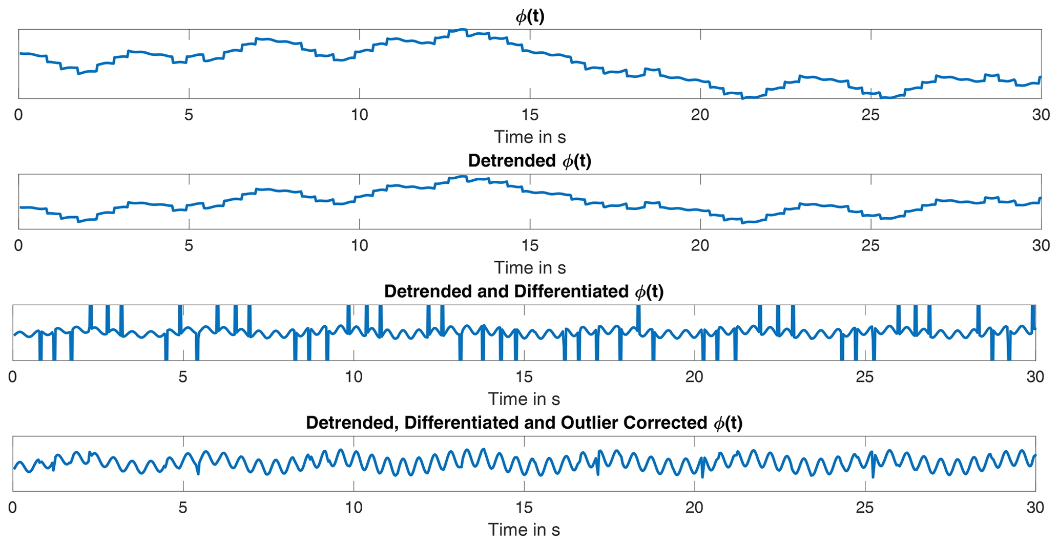
Therefore, the radar voltage signal of each frequency ramp is transferred into the frequency domain via FFT for classical range processing. Prior, the signal is windowed with a Hann-window to suppress leakage and zero-padded to generate a larger amount of supporting points. This is done for all individual ramps separately. By determining the signal's peak in the frequency domain the corresponding frequency can be extracted which belongs to the observed two-body model. Quickly, it is apparent that there is only one peak in the frequency domain and not two, although the two-body model certainly consists of two targets in the radar's line of site. Both targets are so close to each other, their frequency lobes blur into one lobe and are not distinguishable. This is attributable to the resolution of a radar using a bandwidth of f_δ=250 MHz. The minimum resolution is Δ_R min≈0.6 m, which is far from the two body's distance which is ranging in a single digit centimetre area. Hence, to track the movement due to heartbeat and respiration in the millimetre and centimetre range the pure result of the FFT is not sufficient. When observing the progression of the radar response within consecutive ramps, it is noticeable that those are slightly phase shifted to each other. This phase shift is caused by the slightest movements of the two-body model, this phase-shift is accessible by interpreting the frequency domain signal's phase. From the first ramp, the bin with maximum peak in frequency domain (absolute values) is noted, the value of the phase in the frequency domain at this bin is saved. For the next ramp the phase value at this bin is also saved to this vector as for every following ramp. The phase rises and falls over time corresponding to the targets' movement opening and closing to the radar. This creates a new time-domain signal ϕ(t). The phase progression ϕ(t) is the result of the overlaid distances and movements. Only the respiration movement is vivid in the original not further processed ϕ(t).

The phase data is massively corrupted by fast alterations almost looking like points of discontinuity, making the signal noisy and tough to analyse. These points originate from the superposition of both bodies and their phase shift. An easy way to expose the discontinuities in ϕ(t) is by differentiating the signal with respect to the time. The fast alterations in ϕ(t) are significant peaks in $\dot{\mathit{\varphi }}\left(t\right)$. Yet, the other oscillations keep their frequencies. The noisy peaks are vividly identifiable as not being part of the continuous signal of $\dot{\mathit{\varphi }}\left(t\right)$. The main part of $\dot{\mathit{\varphi }}\left(t\right)$ is located in a limited interval. With the outlier test by Grubbs featuring the generalized extreme Studentized distribution (GESD-test) it is possible to detect data points which appear not to fit to the majority. The GESD-test is an statistical, iteratively applied outlier test for a data series x, based on the Grubbs test. The test detects outlier depending on the t-distribution, also known as Student's t-distribution, and a defined threshold. In advantage to the Grubb's and Tietjen-Moore test the number of outliers is not known in advance for the GESD test and it performs better when two or more outlier follow each other consecutively (Grubbs, 1950; NIST, 2012).

In detail the GESD-test works as follows: The data vector x is checked for outliers. The vector x with its length N changes in every iteration, that is, it is denoted with the iteration number k. First, the the value R_k of the N−k-length data vector x_k is calculated (Eq. 1), here σ_x is the standard deviation and μ_x the mean value of x. The data point of x_k that maximizes Eq. (1) is the examined data point n_k and potential outlier.

$$\begin{array}{}\text{(1)}& R_k={\displaystyle \frac{\text{max}\mathrm{|}{\mathit{x}}_k-{\mathit{\mu }}_x\mathrm{|}}{{\mathit{\sigma }}_x}}\end{array}$$

Following α is defined to set the significance level. The value of $\mathit{ϵ}=N-k-\mathrm{1}$ varies in each iteration, too. The value of ϵ defines the t-distribution (Eq. 2), whereby ϵ represents the distribution's degree of freedom and Γ the gamma function.

$$\begin{array}{}\text{(2)}& f\left(t\right)={\displaystyle \frac{\mathrm{\Gamma }\left(\frac{\mathit{ϵ}+\mathrm{1}}{\mathrm{2}}\right)}{\sqrt{\mathit{ϵ}\mathit{\pi }}\mathrm{\Gamma }\left(\frac{\mathit{ϵ}}{\mathrm{2}}\right)}}{\left(\mathrm{1}+{\displaystyle \frac{t^{\mathrm{2}}}{\mathit{ϵ}}}\right)}^{-\frac{\mathit{ϵ}+\mathrm{1}}{\mathrm{2}}}\end{array}$$

The probability value p is defined as in Eq. (3).

$$\begin{array}{}\text{(3)}& p=\mathrm{1}-{\displaystyle \frac{\mathit{\alpha }}{\mathrm{2}\mathit{ϵ}+\mathrm{4}}}\end{array}$$

The value of t_p,ϵ is the 100p percentage point from the t-distribution from the kth iteration. Eventually, the threshold ξ is calculated (Eq. 4).

$$\begin{array}{}\text{(4)}& {\mathit{\xi }}_k={\displaystyle \frac{(N-k)t_{p,\mathit{ϵ}}}{\sqrt{(\mathit{ϵ}+t_{p,\mathit{ϵ}}^{\mathrm{2}})(\mathit{ϵ}+\mathrm{2})}}}\end{array}$$

If Eq. (5) is true, the data sample n_k is classified as outlier and removed. The algorithm restarts with N−k samples respectively. If Eq. (5) is false, n_k is not an outlier and there are no (further) outlier in the dataset, the GESD test is completed (Grubbs, 1950; NIST, 2012)

$$\begin{array}{}\text{(5)}& R_k>{\mathit{\xi }}_k\end{array}$$

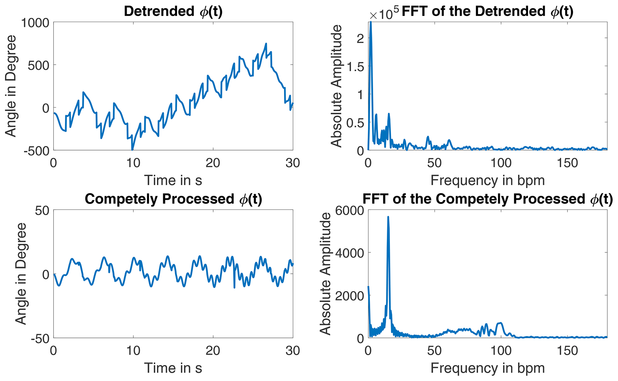
The detected outliers are replaced with interpolated data by using a fitted chirp signal. The processing of the signal is shown in Fig. 1. This signal appears to be pure, as both oscillations due to heartbeat and respiration are already identifiable. The exact angle information gets lost due to the processing. Its frequency spectrum shows a clear peak for the respiration and a several swings in the heartbeat rate region, see Fig. 2.

The wavelet transformation is chosen to separate both vital sign signals in ϕ(t) since it performs signal analysis and synthesis in different frequency ranges simultaneously. In comparison to a common short-time Fourier analysis the wavelet transformation serves with a better frequency resolution at lower frequencies and further a better time resolution at higher frequencies. The wavelet analysis fits best for signals interrupted by discontinuities, while usually having a smooth progression and for signals that superimpose each other despite being in different frequency ranges, both is the case in this application.

Figure 1 Different stages of the phase signal's processing.

Figure 2 Example for frequency spectra of unprocessed and fully processed phase data ϕ(t).

The wavelet transformation is a time-frequency analysis based on filtering. It serves for signal analysis, filtering and synthesis. Its foundation is the use of multiple scaled window functions and time shifting. A wavelet ψ(t) is a zero-mean window function with an average frequency f_ψ≠0. A not scaled or time shifted wavelet is called mother wavelet. Scaling with a and time shifting with b, as in Eq. (6) with $a,b\in {\mathbb{R}}^{+}$, modifies the wavelet ψ_a,b for the later applied wavelet analysis.

$$\begin{array}{}\text{(6)}& {\mathit{\psi }}_{a,b}\left(t\right)={\displaystyle \frac{\mathrm{1}}{\sqrt{a}}}\mathit{\psi }\left({\displaystyle \frac{t-b}{a}}\right)\end{array}$$

Bandwidth Δ_f and time duration Δ_t of the transform are heavily depending on a. The factor $\frac{\mathrm{1}}{\sqrt{a}}$ secures a constant signal energy of any scaled wavelet. The result of the wavelet transform are the wavelet coefficients. While the average time is τ=b and the average frequency is $f=\frac{f_{\mathit{\psi }}}{a}$. A small a leads to fine frequency resolution at high frequencies, large a can perform a fine frequency resolution at low frequencies. Any wavelet function ψ(t) and its corresponding frequency transform Ψ(f) must satisfy (Eq. 7).

$$\begin{array}{}\text{(7)}& \underset{\mathrm{\infty }}{\overset{\mathrm{\infty }}{\int }}{\displaystyle \frac{\mathrm{|}\mathrm{\Psi }\left(af\right){\mathrm{|}}^{\mathrm{2}}}{\mathrm{|}f\mathrm{|}}}<\mathrm{\infty }\end{array}$$

Is Eq. (7) true, fulfils the wavelet transform the Parseval energy conservation. The wavelet transform $W_x^{\mathit{\psi }}(a,b)$ of a signal x(t) is performed with Eq. (8).

$$\begin{array}{}\text{(8)}& W_x^{\mathit{\psi }}(a,b)={\displaystyle \frac{\mathrm{1}}{\sqrt{a}}}\underset{\mathrm{\infty }}{\overset{\mathrm{\infty }}{\int }}x\left(t\right)\mathit{\psi }\left({\displaystyle \frac{t-b}{a}}\right)\mathrm{d}t\end{array}$$

A time shift t_s in x(t−t_s) shifts the wavelet transform by the same time $W_x^{\mathit{\psi }}(a,b-t_{\mathrm{s}})$, hence the wavelet transform is invariant for a time shift. Also the wavelet transform is invariant in scaling, a function is scaled with s as $\frac{\mathrm{1}}{\sqrt{\mathrm{|}s\mathrm{|}}}x\left(\frac{t}{s}\right)$ the transform is scaled, too: $W_x^{\mathit{\psi }}\left(\frac{a}{s},\frac{b}{s}\right)$ (Percival and Walden, 2000; Kienecke et al., 2008).

To benefit the wavelet transform's potential to resolve good frequency resolutions in high as in low frequencies, the transform is performed multiple times (K-times) with differing a and b. The scale factor a is usually chosen dyadic as a_k=2^k with $k=\mathrm{1},\mathrm{2},\mathrm{\dots }K$. The time scale factor b rises dyadic, too, $b_{k,m}={\mathrm{2}}^{k}mT$, that is, the sample distance of the wavelet coefficients are further apart for wavelets with a higher k. The analysing wavelet ψ_k(t) is calculated dyadic as in Eq. (9).

$$\begin{array}{}\text{(9)}& {\mathit{\psi }}_k\left(t\right)={\mathrm{2}}^{-\frac{k}{\mathrm{2}}}\mathit{\psi }({\mathrm{2}}^{-k}t-mT)\end{array}$$

The wavelet transform at (m,k) is then $W_x^{\mathit{\psi }}(m,k)=W_x^{\mathit{\psi }}\left(m{\mathrm{2}}^{k}T,{\mathrm{2}}^k\right)$ with $W_x^{\mathit{\psi }}$ as in Eq. (8).

In general, a wavelet is characterized as bandpass-filter. For a k the wavelet transform projects x(t) in a subspace with the frequencies $]{\mathrm{2}}^{-k}{F}_{\mathrm{N}},{\mathrm{2}}^{-k+\mathrm{1}}{F}_{\mathrm{N}}]$, whereby F_N is the Nyquist frequency. The projection results in a function y_k(t). For the original signal x(t) and its projections y_k(t) take Eqs. (10) and (11) affect. The signal x_k(t) takes the low-pass parts of $x\left(t\right)\widehat{=}{x}_{k-\mathrm{1}}\left(t\right)$ which are below the bandpass-subspace of y_k(t). Equations (10) and (11) show the mathematical connection of x(t), x_k(t) and y_k(t) with $\overline{x}\left(t\right)$ representing x(t) in the relevant frequency domain of [F_N 0].

$$\begin{array}{}\text{(10)}& {\displaystyle }\overline{x}\left(t\right)=x_{\mathrm{0}}\left(t\right)=\sum _{k=\mathrm{1}}^{\mathrm{\infty }}\sum _{m=\mathrm{1}}^{\mathrm{\infty }}{W}_x^{\mathit{\psi }}(m,k){\mathit{\psi }}_{m,k}\left(t\right)=\sum _{k=\mathrm{1}}^{\mathrm{\infty }}{y}_k\left(t\right)\text{(11)}& {\displaystyle }{x}_{k-\mathrm{1}}\left(t\right)=x_k\left(t\right)+y_k\left(t\right)\end{array}$$

These coherence can also be expressed in their subspaces. For a function x(t)∈L₂(ℝ), with L₂(ℝ) being the subspace of all square-integrable functions, is y_k(t) the projection in the subspace W_k while x_k(t) is part of the low-pass subspace V_k. The subspaces have the coherences Eqs. (12) and (13).

$$\begin{array}{}\text{(12)}& {\displaystyle }{V}_{k-\mathrm{1}}=V_k\cup W_k\text{(13)}& {\displaystyle }{V}_k\cap W_k=\oslash \end{array}$$

The transition from V_k−1 to W_k is performed by a bandpass filter G_BP with the impulse response g_BP(m), and from V_k−1 to V_k by a low-pass filter G_LP with the impulse response g_LP(m). The subspace V_k is spanned by the orthonormal base function ${\mathit{\varphi }}_{m,k}\left(t\right)={\mathrm{2}}^{-\frac{k}{\mathrm{2}}}\cdot \mathit{\varphi }({\mathrm{2}}^{-k}t-mT)$ which is orthogonal to the wavelet ψ_m,k(t) for all m,k. The base function ψ is also called scale function and is able to describe x_k(t) in V_k.

$$\begin{array}{}\text{(14)}& x_k\left(t\right)=\sum _{m=\mathrm{0}}^{\mathrm{\infty }}\langle x_{k-\mathrm{1}}\left(t\right){\mathit{\varphi }}_{m,k}\left(t\right)\rangle \cdot {\mathit{\varphi }}_{m,k}\left(t\right)\end{array}$$

When transitioned into another subspace the impulse responses g(t), wavelet ψ_k+1(t) and scale functions ψ_k(t) and ψ_k+1(t) are related with Eq. (15).

$$\begin{array}{}\text{(15)}& \begin{array}{rl}{\mathit{\varphi }}_{m,k}\left(t\right)=& \sum _{l=m-\mathrm{\infty }}^{\mathrm{\infty }}{g}_{\text{TP}}(\mathrm{2}l-m){\mathit{\varphi }}_{l,k+\mathrm{1}}\\ & +\sum _{l=m-\mathrm{\infty }}^{\mathrm{\infty }}{g}_{\text{BP}}(\mathrm{2}l-m){\mathit{\psi }}_{l,k+\mathrm{1}}\end{array}\end{array}$$

The argument 2l−m needs some closer attention, increasing the index of ψ_k+1(t) and ψ_k+1(t) by one, increases the index in ψ_k(t) by two. Consequently, the subspace V_k+1 and W_k+1 are sampled with halve the sample frequency as V_k. For the inverse wavelet transformation besides the scale and wavelet function the impulse responses $h_{\text{BP}}\left(m\right)=g_{\text{BP}}^{*}(-m)$ and $h_{\text{LP}}\left(m\right)=g_{\text{LP}}^{*}(-m)$ and their corresponding filters are needed. Eventually, to determine the filter bank only h_LP is needed from the start. The other filter and their responses can be calculated with h_LP, the bandpass filter response is $h_{\text{BP}}\left(m\right)=(-\mathrm{1}{)}^m{h}_{\text{BP}}^{*}(\mathrm{1}-m)$. The low pass filter H_LP and its response h_LP are used to calculate the scale function ψ(t) and the wavelet function ϕ(t), too.

$$\begin{array}{}\text{(16)}& \mathit{\varphi }\left(t\right)={\displaystyle \frac{\mathrm{1}}{\mathrm{2}\mathit{\pi }}}\underset{-\mathrm{\infty }}{\overset{+\mathrm{\infty }}{\int }}\prod _{k=\mathrm{1}}^{\mathrm{\infty }}\left({\displaystyle \frac{\mathrm{1}}{\sqrt{\mathrm{2}}}}{H}_{\text{LP}}\left({\displaystyle \frac{f}{{\mathrm{2}}^k}}\right)\right){\mathrm{e}}^{\mathrm{2}\mathit{\pi }jft}\mathrm{d}t\end{array}$$

With the low pass filter response h_LP and the scale filter ϕ(t) the wavelet function ψ is calculated in Eq. (17).

$$\begin{array}{}\text{(17)}& \mathit{\psi }\left(t\right)=\sum _{m=-\mathrm{\infty }}^{\mathrm{\infty }}(-\mathrm{1}{)}^m{h}_{\text{LP}}^{*}(\mathrm{1}-m\left)\sqrt{\mathrm{2}}\mathit{\varphi }\right(\mathrm{2}t-mT)\end{array}$$

The previously described fully processed ϕ(t) is used for the transformation. Used are the MATLAB-functions modwt and modwtmra for transformation and analysis. A Symlet-4 is utilized as wavelet and its corresponding scaling function. The wavelet transformation level is 7, following a sample frequency of f_rr the signal is divided in frequency intervals as in Table 1 (Percival and Walden, 2000; Kienecke et al., 2008; MathWorks, 2020).

Table 1 Frequency intervals according to the described wavelet transformation, values are rounded, the residue is omitted.

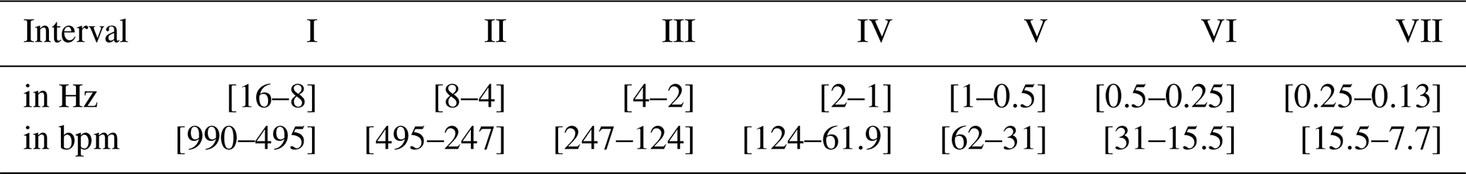
For the respiration frequency intervals VI and VII are to consider, satisfying the respiration rate in a range of 12 to 20 respirations per minute. For the pulse the interval IV is sufficient for the simulation. Although cutting the heartbeat frequency off at 124 bpm which is sufficient for the simulated data. The wavelet coefficients are processed to synthesize the original signal in the corresponding frequency bounds. For the respiration signals the intervals VI and VII are summed up, baseline wander can be removed easily (Kienecke et al., 2008; MathWorks, 2020).

The frequency in the separated signals is estimated with the root-MUSIC. The root-MUSIC is a variant of the MUSIC algorithm, which is a frequency estimation method based on the fundamentals of Pisarenko's harmonic decomposition. It was first presented by Arthur J. Barabell in 1983. The pivotal step is to split the correlation matrix' R_x eigenvectors λ in a signal subspace and noise subspace (Manolakis et al., 2005; Barabell, 1983).

For the Root-MUSIC algorithm some knowledge about the evaluated signal x(t) is needed: that is the signal length M and more crucial the number of contained harmonic oscillations P. For the root-MUSIC algorithm $M>P+\mathrm{1}$ must be true, that means the evaluated time window of x(t) must be at least contain two more samples than harmonic oscillations. The signal x(t) is assumed to be the sum of the actual signal s(t) and uncorrelated white noise w(t). x(t) can be denoted as Eq. (18), whereby the vector v(f) is the frequency vector in form of a M-length DFT-vector.

$$\begin{array}{}\text{(18)}& x\left(t\right)=s\left(t\right)+w\left(t\right)=\sum _{p=\mathrm{1}}^P{\mathit{\alpha }}_p\mathit{v}\left(f_p\right)e^{j\mathrm{2}\mathit{\pi }t{f}_p}+\mathit{w}\left(n\right)\end{array}$$

Similar to the time signal itself the autocorrelation R_x can be split into signal R_s and noise correlation matrices R_s, assuming independence of signal and noise. The autocorrelation may also be expressed with eigenvalues λ and their respective eigenvectors q, as defined in Eq. (19).

$$\begin{array}{}\text{(19)}& {\mathbf{\text{R}}}_x=E\mathit{\left\{}x\right(n\left)x^H\right(n\left)\mathit{\right\}}={\mathbf{\text{R}}}_{\mathrm{s}}+{\mathbf{\text{R}}}_w=\sum _{k=\mathrm{1}}^M{\mathit{\lambda }}_k{\mathit{q}}_k{\mathit{q}}_k^H\end{array}$$

The eigenvalues are sorted in descending order, that ${\mathit{\lambda }}_{\mathrm{1}}\ge {\mathit{\lambda }}_{\mathrm{2}}\ge \mathrm{\dots }\ge {\mathit{\lambda }}_M$ is true. For m>P the eigenvalues λ_k are caused by noise and can be summarized in ${\mathit{\sigma }}_w^{\mathrm{2}}$. For k≤P the eigenvalues λ_k are evoked by the actual signal s(t). The subspaces of signal and noise are orthogonal following is the frequency vector v^H(f_p) orthogonal to Q_w with ${\mathbf{\text{Q}}}_w=\left[{\mathit{q}}_{P+\mathrm{1}}\mathrm{\dots }{\mathit{q}}_M\right]$. The pseudospectrum ${\stackrel{\mathrm{‾}}{R}}_m$ for one eigenvector q_k calculates to:

$$\begin{array}{}\text{(20)}& {\stackrel{\mathrm{‾}}{R}}_k\left(e^{j\mathrm{2}\mathit{\pi }f}\right)={\displaystyle \frac{\mathrm{1}}{\mathrm{|}{\mathit{v}}_H\left(f\right){\mathit{q}}_k{\mathrm{|}}^{\mathrm{2}}}}\end{array}$$

The denominator of Eq. (20) produces M−1 roots, M−P of them due to the noise subspace and occur on different frequencies without any restrictions. However, P of them are correspond to the P oscillations in s(t). To secure a correct identification of peaks corresponding to the frequencies f_P, the MUSIC-pseudospectrum ${\stackrel{\mathrm{‾}}{R}}_{\text{MUSIC}}$ is defined as in Eq. (21).

$$\begin{array}{ll}{\displaystyle }{\stackrel{\mathrm{‾}}{R}}_{\mathrm{MUSIC}}\left(e^{j\mathrm{2}\mathit{\pi }f}\right)& {\displaystyle }={\displaystyle \frac{\mathrm{1}}{{\sum }_{k=P+\mathrm{1}}^M\mathrm{|}{\mathit{v}}_H\left(f\right){\mathit{q}}_k{\mathrm{|}}^{\mathrm{2}}}}\\ \text{(21)}& {\displaystyle }& {\displaystyle }={\displaystyle \frac{\mathrm{1}}{{\sum }_{k=P+\mathrm{1}}^M\mathrm{|}{\mathbf{\text{Q}}}_k\left(e^{j\mathrm{2}\mathit{\pi }f}\right){\mathrm{|}}^{\mathrm{2}}}}\end{array}$$

The peaks of ${\stackrel{\mathrm{‾}}{R}}_{\mathrm{MUSIC}}$ represent the frequencies f_P. For the root-MUSIC approach the z-transform of the denominator in Eq. (21) is needed, Eq. (22) represents the sum of the noise vector's pseudospectrum in the z-domain.

$$\begin{array}{}\text{(22)}& P\left(z\right)=\sum _{k=P+\mathrm{1}}^M{\mathbf{\text{Q}}}_k\left(z\right){\mathbf{\text{Q}}}_k^{\ast }\left({\displaystyle \frac{\mathrm{1}}{z^{\ast }}}\right)\end{array}$$

From Eq. (22) stem M−1 pairs of roots with one inside and one outside the unit circle. Since there is no attenuation on the P oscillations, the P-closest roots to the unit circle match the oscillations in s(t). For real signals x(t)=Re(x(t)) with k frequencies f_k, P=2k roots have to be regarded. Due to the two sided spectrum the roots appear at each f_k and at −f_k (Manolakis et al., 2005; Barabell, 1983).

3 Off-Line Processing for Real-World Data

The two-body model for the simulation is sufficient for a first testing, yet it is not covering the complex movements of the upper body entirely. Further are the altering variables, such as the heartbeat rate, really complex to model as they follow no known rule and are more like a mathematical chaos. The simulation of their shift is a simple approximation. To proceed with the algorithm development it is tested with real data. The data is measured with a radar working under the same settings as the simulation except for the sampling rate, which is slower, and the ramp repetition frequency, which is faster. Each measurement is 3 min in time. Several test persons were used for the measurement procedure, in some cases they were given special tasks such as holding their breath for a period of time. All have a healthy respiration system. For later comparison the monitored persons are connected to an ECG which tracks the heartbeat data parallel.

Before starting the vital sign calculation, the phase progression ϕ(t) is extracted as described in the previous section. The reconstructed signals for both vital signs there is a noticeable differing in their frequency and amplitude over time which is distinctly higher than in the simulation. The oscillations appear uneven as there are flatter and steeper parts in the phase progression. The signal processing algorithm developed for the simulated signals fails, especially for the heartbeat. Errors between the ECG-data are significant and not tolerable. Hence the algorithm is further developed and the input signal analysed.

In comparison to the simulated two-body model the signal ϕ(t) is derived from the chest movement affected by considerably more radar targets as neither the chest nor the abdomen can be considered as uniformly moving unit. The movement amplitude is differing on the various upper body parts. Additionally, besides the movements due to heartbeat and respiration other irregular motions are to expect, although the test person were told to sit still and not to talk. In sum this certainly leads to a less smooth phase progression as in the simulation with more superimposed intermittent oscillations. Since the wavelet transform's resolution already causes problems in analysis of the simulation an improved version of the wavelet transformation is chosen for the further development: The wavelet packet transform. For most applications in signal processing is it useful to have the targeted frequency parts in preferably few subspaces. Yet, especially in higher frequency ranges the frequency bandwidth can be quite huge, while the short time resolution in those is not essential if the signal is fairly stable in its frequency over time. This issue can be solved by using wavelet packets. In the regular wavelet transformation the subspaces V_k and W_k are strictly expanded from the previous low-pass subspace V_k−1. Thus, the bandpass subspace W_k is not further processed. The subspaces in the wavelet packet transformation are expanded in both V_k and W_k. That is, the signal y_k(t) is transformed, too. For k=1 is no difference to the standard wavelet transformation, but if k=2 there are 4 subspaces present. The indice i is introduced along with k:

• V_2,0 the low-pass subspace of V₁ containing x_2,0(t)

• W_2,1 the band-pass subspace of V₁ containing y_2,1(t)

• V_2,2 the low-pass subspace of W₁ containing x_2,2(t)

• W_2,3 the band-pass subspace of W₁ containing y_2,3(t)

For larger k the time resolution becomes worse, yet the frequency resolution improves. By a constant k signals and subspaces with higher i represent higher frequency bandwidths (Kienecke et al., 2008).

This transform is capable to realize an even resolution distribution of the individual frequency intervals. The frequency width of a single interval (or level) is depending on the chosen tree depth. To achieve a desired resolution, the tree-depth is chosen to 9 which results in 512 nodes. By a radar ramp repetition frequency of 62.5 Hz the frequency levels have a width of 0.061 Hz (3.662 bpm). MATLAB provides two functions to perform a complete transform with wavelet filter banks: modwpt ensures an accurate resolution of the energy to the frequency levels, drawback is a delay in the time domain for the wavelet coefficients. This effects arises from the use of filters with a non-linear phase response. While the other function modwptdetails is true to the time, which is particularly important for the signal synthesis. In opposite to the other this function utilises zero-phase filtering for the transformation, which is mandatory for the application.

The frequency may be estimated from a time domain signal, therefore the wavelet coefficients are regarded, which represent the original signal in the respective frequency level. For this transformation the function modwptdetails is used. Since the exact value is yet to be determined, the whole pulse related possible frequency range is regarded. That is, the levels 14–49 contain frequencies in the interval of 0.824–3.021 Hz (49.44–181.27 bpm). Therefore, the coefficients of these levels are summed up. This signal equals the original signal in the corresponding frequency bounds.

For heartbeat estimation is the signal cut into 3 s parts. The consequently following data snippet is reconstructed in dependence to the previously detected heartbeat rate. Only adjacent frequency levels of the one containing the heartbeat are regarded, limiting the evaluated frequency interval to 0.31 Hz (18.6 bpm). With the reconstruction being a simple summation of wavelet coefficients, it is easy to handle for each data excerpt.

Since the phase progression appears to be less harmonic and the oscillations' frequency and amplitude differs massively, the estimation with root-MUSIC causes issues. The number of frequencies in a signal processed with root-MUSIC must be known precisely. If the signal or the evaluated signal part is corrupted due to minor body movement the estimated frequency can deviate from the correct heartbeat frequency massively. Hence, the data is searched progressively for erratic oscillations with the Pearson-Coefficient. If a fitting part is not detected, it is omitted. Nevertheless, outlier occur those are ascertained and removed by the Grubbs test for outlier and afterwards replaced by interpolation. An example for excluded data is shown in Fig. 3.

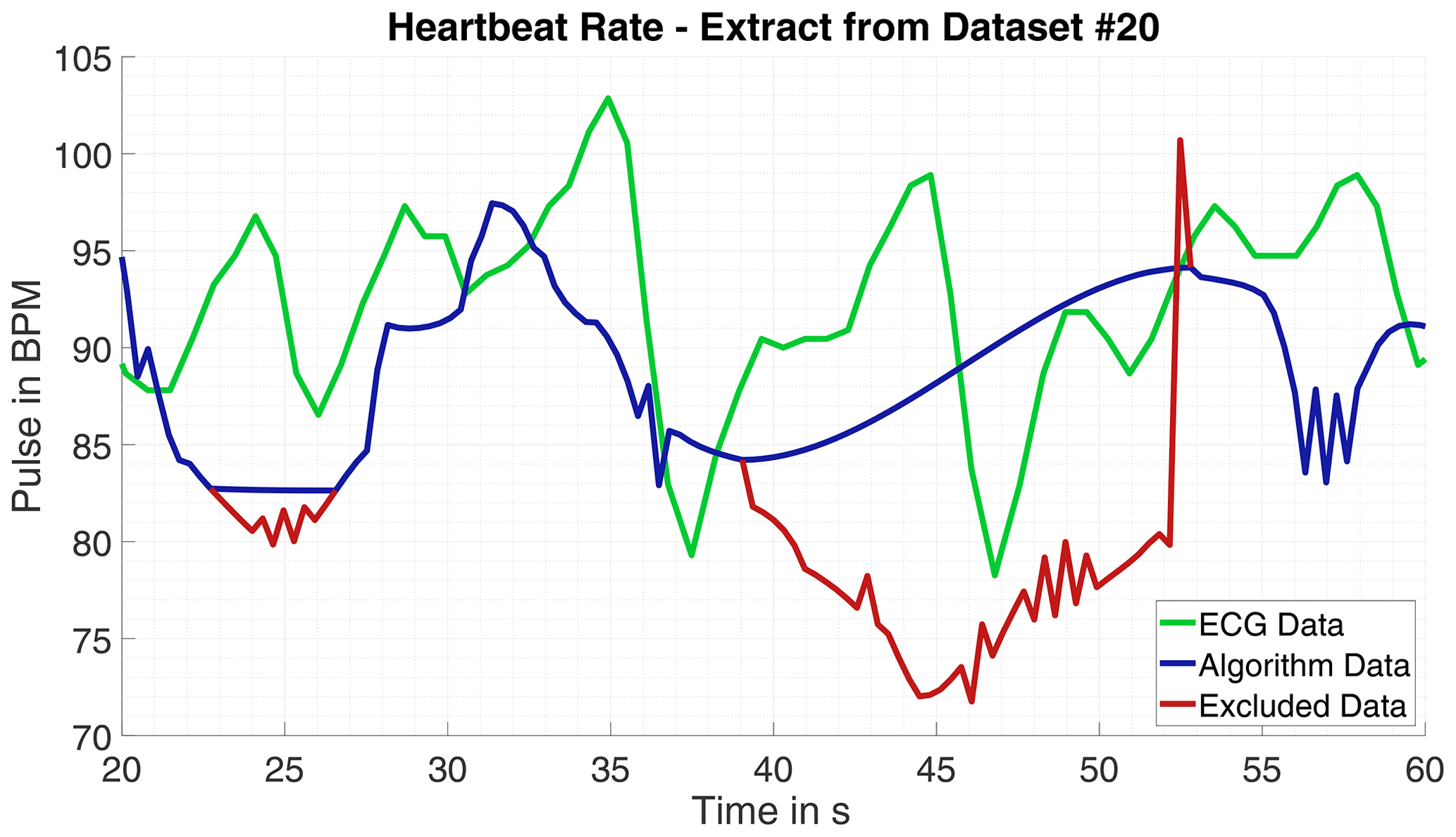
Figure 3 Heartbeat rate for ECG and radar data inclusive omitted data due to statistical outlier.

For the detection of the respiration movement and consequently the respiration rate the same input data is used as for the heartbeat rate. The processing is similar to the heartbeat detection. The data is differentiated before wavelet transformed, too. The relevant frequency interval is lower and overall smaller as for the heartbeat, yet the level frequency width is chosen the same with 0.061 Hz. That is, the wavelet packet transform must be performed only once to calculate both vital signs. The respiration is assumed in the frequency range of 12 to 20 breaths per minute. Thus, the levels 2 to 6 are used for signal reconstruction, with the signal having frequencies in the bounds of 0.09–0.40 Hz (5.5–23.8 bpm). For the time signal analysis the sliding time window is adjusted to the slower frequencies, too. The window size is 500 sample points (8 s of data), this time window should be sufficient to have one full breathing cycle within, even for slow respiration rates. The time step for each evaluated data excerpt is set to 1.92 s, the alterations in the respiration are expected to be not as sudden as for the heartbeat. The sample frequency of the generated respiration signal following the time step length is roughly 0.5 Hz.

3.1 Results

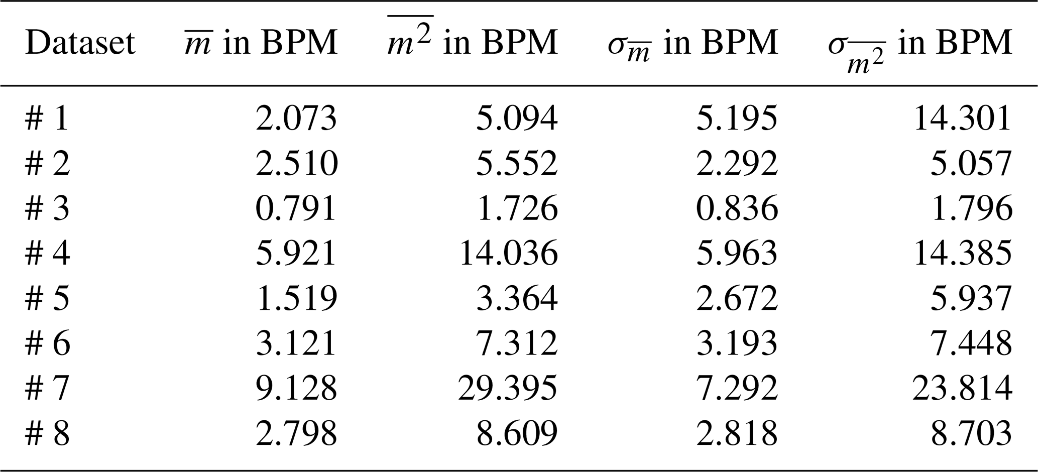
Having the gold-standard of heartbeat frequency measurement electrocardiography as reference is the best case scenario to evaluate the algorithm results. Observing the error over time m(t) for all measurements are significant deviations partially only for a few seconds noticeable. Looking closely into the data for some parts massive outlier are recognizable, for example in one measurement the ECG calculated heartbeat frequency rises tremendous two times for 2 s peaking at over 220 bpm and falling then back to plausible values. This happens into unnatural deep ranges, too, in another measurement the ECG calculated pulse falls from 90 below 40 within seconds before rising again. Those miscalculations by the ECG may not compromise the quality of the radar based pulse computation. Therefore, the error is calculated once more with the intervals of implausible ECG-data omitted. With this approach the average absolute error over all measurements is $\stackrel{\mathrm{‾}}{m}=\mathrm{3.138}$ bpm with a standard deviation of σ=2.839 bpm. The results of one single measurement and comparison to ECG-data is shown in Fig. 4 and in numbers for eight measurements in Table 2.

Table 2 Errors and standard deviations for all measurements for complete datasets and modified data with ECG-data anomalies and possible background movements automatically cut out.

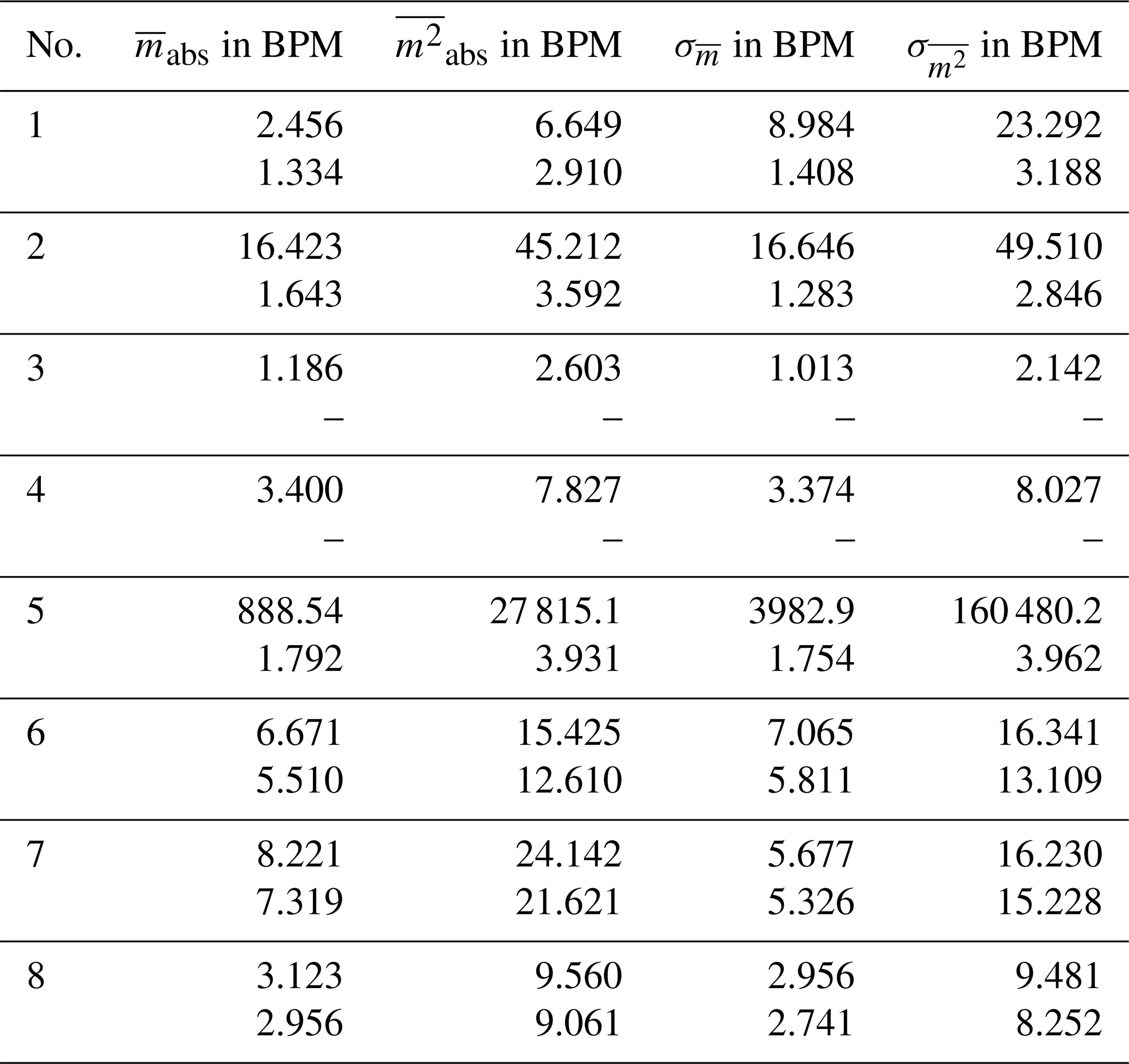
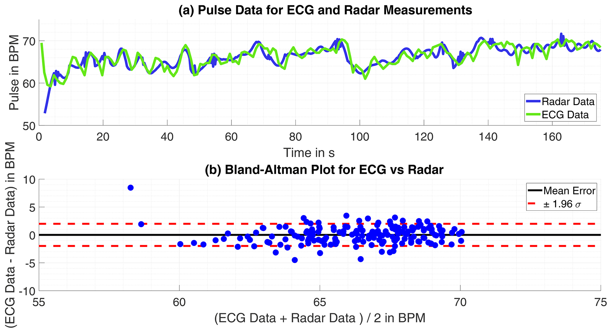
Figure 4 (a) Time progression of the heartbeat tracked by ECG and radar. (b) Bland-Altman Plot for both approaches.

On the first look, the respiration rate calculated with the radar-data is plausible. The respiration has some dynamic over time and yet no discontinues are to find. Only smaller spikes strike arise, these could be avoided by applying a low-pass filter, as a moving-average filter, with the drawback of more time-inertial. However, within some of the datasets the monitored persons were told to hold the breath for a certain time. These parts of respiratory arrest are not correctly detected at all. The reason for that failure are apparent, the wavelet level of very low frequencies, below 0.09 Hz (5.5 bpm), are excluded to avoid wrong detections at first. In this region is a lot of noise which would disturb the frequency estimation. Additionally forces the frequency estimation with the root-MUSIC algorithm a detection of a single frequency within a signal, although there is none with significant energy. The estimation treats the oscillations equal not regarding their energy. If the monitored person does not move its chest in the observed frequency range, a phase variation signal within the range will be classified as respiration movement and then estimated as respiration frequency. The mean error for the 4 datasets without respiratory standstill is m=1.92 bpm (0.032 Hz) and the standard deviation σ_m=1.21 bpm (0.020 Hz). A Bland-Altman plot showing the results in comparison to the ECG-data is given in Figs. 5 and 6.

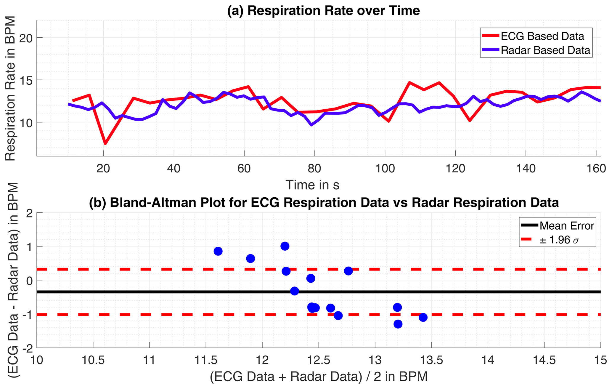
Figure 5 (a) Time progression of the respiration rate tracked by ECG and radar. (b) Bland-Altman Plot for both approaches.

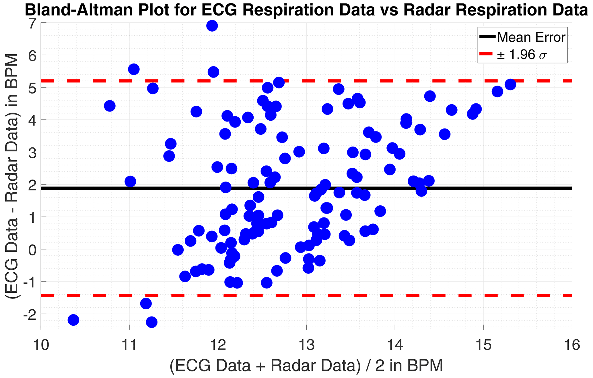
Figure 6 Bland-Altman Plot for the respiration rate measurements comparing ECG and radar based data.

4 Live Processing for Real-World Data

Vital sign measuring is most importantly done to trace the data in a live measurement as the data is needed immediately for further diagnosis. Therefore, the given measurement sets are processed pseudo-live, that is, the signal is partially loaded to the algorithm in real time. In opposite to the initial off-line processing algorithm the data is completely transformed to the wavelet coefficients at the beginning. Since the single level frequency resolution shall not be decreased, the wavelet packet transformation tree depth is unchanged at 9. For the long off-line processed data sequence, this is quite CPU-intensive but once done the coefficients can be used in arbitrary ways without extra computations. In the live algorithm the angle data ϕ(t) is only piecewise processable, hence the wavelet packet transform must be performed several times generating an increase in the calculation time. To ensure proper data sampling and enough calculation time the heartbeat rate here is estimated just every 3.6 s. The short data windows causes another hitch. The wavelet transform is based and bound to different filter, those filter appear to have some settling time as the results of the transform are attenuated at the beginning and the end of the signal. The signal snippet is basically split in thirds. The first and the last third are just dummy data for the processing as the reconstructed signal contains corrupted data in these parts caused by the wavelet transform. That is, only the middle section of the signal part is used for frequency estimation. the latest calculated frequency and the ones already present from former iterations in the heartbeat rate-vector are checked with the GESD test for outlier. As before, detected outlier are replaced by interpolated values. Although tremendous outliers are removed, the heartbeat frequency over time signal appears erratic also it frames the desired values. These leaps are not explainable by heartbeat variations. When observing the derived ECG-signal it is erratic too, yet not to the degree the signal from the radar derived is. In practice, however, the ECG-signal is always averaged over time before it is displayed. Since the ECG is considered the gold-standard of pulse measuring this is a widely held and proven approach. Following, is the heartbeat over time signal derived from the radar measurement averaged over time, just as the ECG-signal, for a fair comparison. Likewise to the extraction from the respiration in off-line processing, the observed time window is enlarged in comparison to the heartbeat detection to fit the appreciable lower frequencies occurring. The lowest in the regarded frequency range frequency has a time period of roughly 10 s, the window size is therefore chosen with a length of 16 s in time.

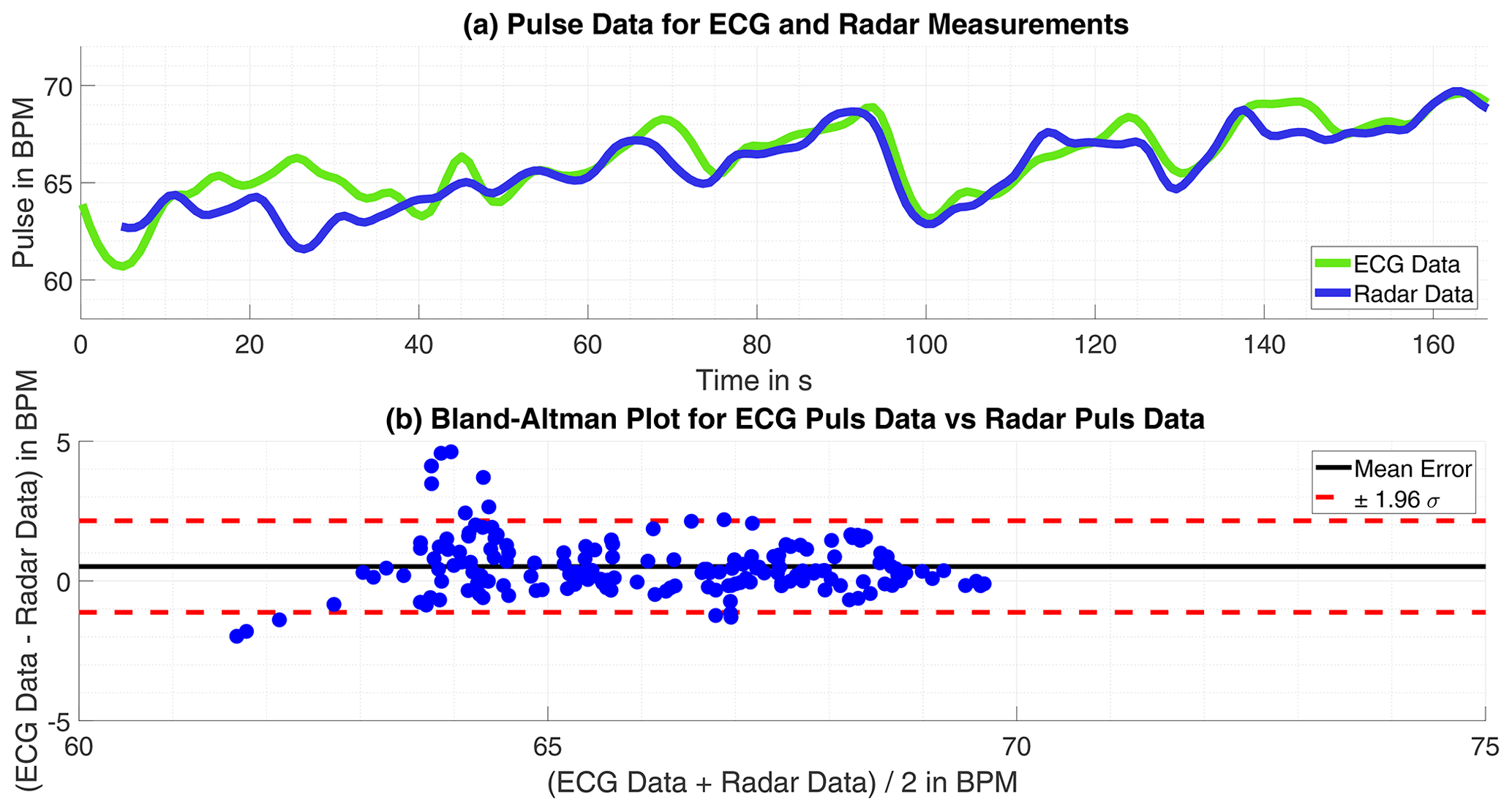
Figure 7 (a) Time progression of the heartbeat tracked by ECG and radar. (b) Bland-Altman Plot for both approaches.

4.1 Results

Eventually the comparison of live processed smoothed data to ECG's data is closer to real-world data since erratic peaks are usually omitted as those are sleeked for evaluation whereas they are assumed as measurement inaccuracy. In opposite to the off-line processed data no extra evaluation, excluding suspected ECG-data measuring errors or disruptive background movement, is done. The time averaged signals are used for comparison, this mitigates the influence of measuring errors to an extend, as single deviations get lost.

Table 3 Statistical errors and their standard deviations for the pseudo-live processed data compared to the ECG-data as reference.

The heartbeat rate only suffer slight errors, larger errors only happened only in time intervals of 5 s or less, but observed throughout the measuring period the result is satisfying. The absolute mean error is $\stackrel{\mathrm{‾}}{m}=\mathrm{3.311}$ bpm with a standard deviation of σ=3.783 bpm. The pure result might be slightly worse than for the off-line processed data but with no probably corrupted ECG failures omitted this is expected and still a fairly good result. Exemplary are the results of one single measurement shown in Fig. 7.

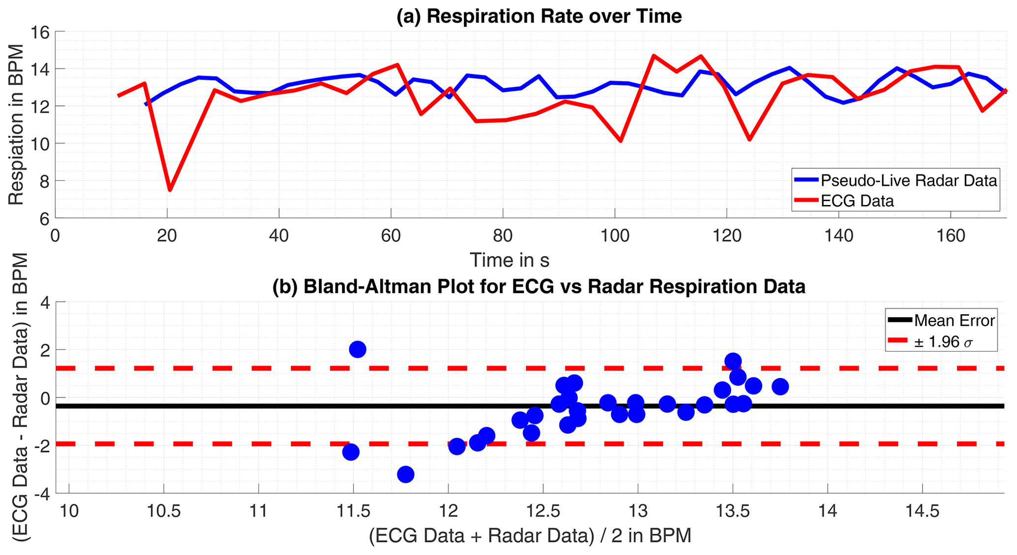
Figure 8 (a) Time progression of the respiration rate tracked by ECG and radar. (b) Bland-Altman Plot for both approaches.

The datasets including a respiratory arrest are excluded from the review, as they are corrupted by measurement failures inevitably. Although the respiration rate's values of both approaches are within the same range and the rate's trend is discernible as similar, the deviations become significant within few intervals. Which is possibly caused by the differing approaches the compared data is acquired.

Overall the mean error is m=1.21 bpm (0.020 Hz) and the standard deviation of the mean error σ_m=1.74 bpm (0.029 Hz), the individual numbers are presented for each measurement in Table (3). This result is satisfying, as the radar delivers respiration rates comparable to the ECG. Partly, the radar data is even more plausible, as it omits rapid variation in the respiration rate, which are tracked in the ECG-data. The comparison is visualized in Figs. 7 and 8.

5 Conclusions

With the lessons learned from the processed simulated data the basics of the algorithm to evaluate data sampled from real humans are quickly established. Yet, other difficulties are encountered as the simulated data lacked in the complexity of the upper body movement and missed common disruptions in the data and measurement noise. The use of correlation, the Pearson-coefficient and the GESD-test helped to overcome those troubles as corrupt data are detected and excluded from the evaluation. For the heartbeat rate, the off-line processing algorithm provided satisfying results overall, when compared to the ECG-data. The estimated respiration rate for all off-line processed datasets is plausible in terms of range and dynamic and follow the same trends as the ECG-data. One major issue for the respiration rate estimation is unavoidably the lack of correct respiratory standstill detection.

Since it is a common approach and consequently closer to the reality the calculated live processed data and the corresponding ECG-data time are averaged before comparison. Here too, the results for the heartbeat rate compared to the ECG-data are satisfying. The impacts of disruptive background movements causes inferior errors than in the off-line processed data, explainable by the larger observed time window and the time averaging. For all datasets without respiratory standstill the results show the working principle is adequate. The slightly larger regarded data time windows in the calculation have no adverse effect on the respiration rate detection. The retrieved data stands comparison to the ECG-data, similar to the off-line processed data. The radar based progression is smoother as it omits rapid variations, making it even more plausible than the ECG-data. The radar trends to detect slightly lower respiration rates, as the deviation between both approaches averages +1.21 bpm (+0.02 Hz).